11. MPO to circuit transpilation

The code executed in this notebook reproduces that of an original paper, which at the same time uses the method from Vidal (note that we reference the first version because it is substantially different from the later versions and contains the appropriate information to follow the procedure).

Other teams built on top of it adding some variants and state preparation in paper 1 and paper 2

---

The goal of this notebook is to illustrate the transpilation of an MPO unitary operator (\(\mathrm{M}_{\mathrm{ref}}\) representing the unitary time evolution induced by some Hamiltonian during a time \(\Delta t\)) into a nearest-neighbor brickwall circuit that can be run on some QPU (\(U_{\mathrm{bw}}\)):

We impose an Ansatz circuit made out of three rows of entangling gates on even-odd-even links. Note that in some references the prescription for increasing the depth/layer counting is just a row of even or of odd entangling gates, while other references consider than two consecutive rows even-odd constitute a layer

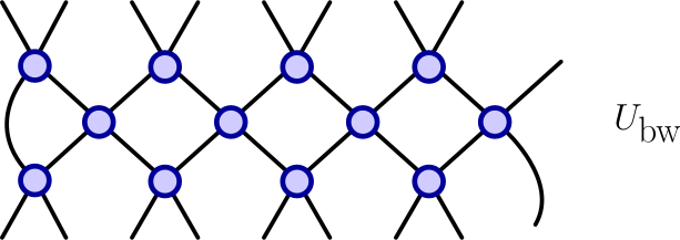
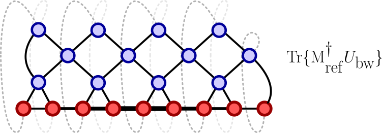
In order to translate the circuit that best reproduces the action of the unitary MPO, we maximize the overlap between the two unitaries. If this cost function is maximized, then \(U_{\mathrm{bw}}\) will act on another state or operator in the same way as \(\mathrm{M}_{\mathrm{ref}}\) does.

In this case, the cost function can be computed as a fully contracted tensor network with a cylindrical topology. An illustration of such a cost function for the formerly introduced ansatz circuit is:

import os

os.environ["NUMBA_NUM_THREADS"] = "1"
os.environ["OMP_NUM_THREADS"] = "1"
os.environ["MKL_NUM_THREADS"] = "1"

import copy

from quimb.tensor import DMRG2

from qpe_toolbox.circuit.mpo_circuit_transpilation import (
    build_first_sweep,
    find_transfer_structure,
    init_cost_tn,
    optimize_single_gate_update,
    state_preparation_mpo,
    trotter_approx_as_MPO,
)
from qpe_toolbox.hamiltonian import Hamiltonian

list_paulis = ["I", "X", "Y", "Z"]

11.1. Dynamics induced by the next-nearest-neighbor Ising model

L = 11
gx, gzz, gz1z = 0.2, 0.5, 0.1
terms_NNIM = []
for x in range(L):
    terms_NNIM.append((gx, "x", [x]))
for x in range(L - 1):
    terms_NNIM.append((gzz, "zz", [x, x + 1]))
for x in range(L - 2):
    terms_NNIM.append((gz1z, "zz", [x, x + 2]))

ham_NNIM = Hamiltonian(terms_NNIM, L)

in the following function: do we keep the verbose? if we keep it, do we change it?

trotter_mpo_ham_NNIM = trotter_approx_as_MPO(
    ham_NNIM,
    order=4,
    dt=0.5,
    cutoff=1e-12,
    max_bond=64,
    verbosity=1,
)

Building 4th order Trotter 

  Building 2nd order Trotter (1st and 3rd layers)
  Building 2nd order Trotter 

    Building 1st order Trotter (1st half)


    Building 1st order Trotter (2nd half)


  Building 2nd order Trotter (2nd layer)
  Building 2nd order Trotter 

    Building 1st order Trotter (1st half)


    Building 1st order Trotter (2nd half)

  Multiplying the 3 MPO layers 

    Final bond dimension: 22

in the following I initialize the cost function

depth = 3

for boundary_bool in [False, True]:
    cost_tn = init_cost_tn(
        ref_mpo=trotter_mpo_ham_NNIM,
        depth=depth,
        param_scaling=1e-1,
        closed=boundary_bool,
    )
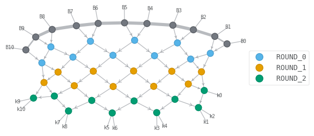
    cost_tn.draw([f"ROUND_{i}" for i in range(depth)], show_inds=True, show_tags=False)

Now we optimize the overlap as suggested in the context of algorithms for entanglement renormalization: to solve the Constrained Linear problem where the isometry to be found decomposes in a given circuit structure, we solve a series of Unconstrained Linear problems for each of the gates forming the circuit. The later is known to have an analytical solution.

The procedure goes as follows: first, we select a given qubit (say, site 0) and target the optimization of all the gates exposed to that qubit. In the following picture we highlight in yellow the set of gates we are referring to:

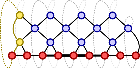
Second, we contract the subnetwork that is not being updated. That contraction is the right environment of qubit 0, \(R_0\); such an environment can be built at the same time from the right environment of qubit 1, \(R_1\), and so until the last qubit:

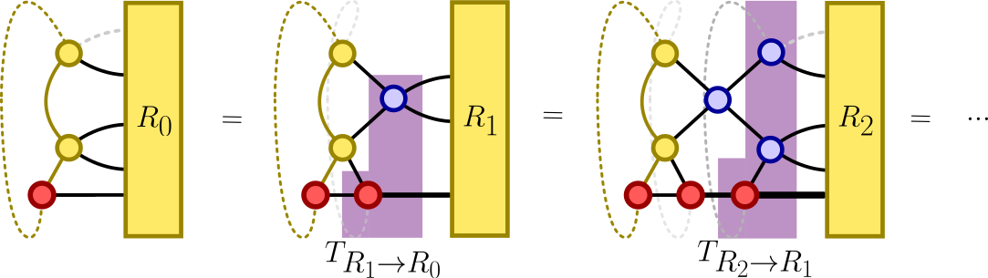
By knowing the first right environment (that of the second-to-last qubit, \(R_{\mathrm{n_qubits-1}}\), which coincides with the last tensor of \(\mathrm{M}_{\mathrm{ref}}\) ) and the tensors required to transfer from one environment to another, we can build all the right environments for the first sweep. Conversely, this can be done for left environments:

dict_transf = find_transfer_structure(n_qubits=L, cost_tn=cost_tn)

dict_contr_envs = build_first_sweep(
    n_qubits=L, cost_tn=cost_tn, dict_transf=dict_transf, drop_tags=True
)

Once the environment structure is found, we need to find the optimal gate to update a particular two-qubit unitary. To do so, we contract all the tensors around it. For example, say we want to update the first unitary at depth 0 between qubits 0 and 1, \(U^{(0)}_{0,1}\); we contract all the tensors around it into its environment \(E^{(0)}_{0,1}\) (this \(E\) environment contains the \(L\) and \(R\) of each site, together with the corresponding tensor from the reference unitary at that site).

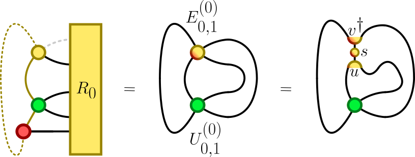
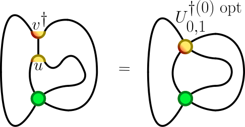
The environment \(E\) is not necessarily a unitary object. To re-introduce unitarity, we can compute the SVD decomposition of it and remove the singular values. This substitution \(E^{(0)}_{0,1} \longrightarrow U^{\dagger (0) \mathrm{opt}}_{0,1}=u v^\dagger\) is indeed the exact analytical solution of the Unconstrained Linear problem:

# note that we optimize for an ansatz the
# "depth" parameters is twice that of Causer et al.

rtol = 1e-6
n_sweeps_max = int(1e2)

cp_cost_tn = cost_tn.copy(deep=True)
cp_dict_transf = copy.deepcopy(dict_transf)
cp_dict_contr_envs = copy.deepcopy(dict_contr_envs)

opt_cost_tn, opt_dict_contr_envs = optimize_single_gate_update(
    n_qubits=L,
    cost_tn=cp_cost_tn,
    rtol=rtol,
    n_sweeps_max=n_sweeps_max,
    dict_transf=cp_dict_transf,
    dict_contr_envs=cp_dict_contr_envs,
)

# retrieve the optimal circuit tensor network
opt_circuit_tn = opt_cost_tn.copy(deep=True)
opt_circuit_tn.delete(tags=("MPO"))

In Causer et al. they find that the model is prone to get stuck on local minima, even when starting from different initial circuits by changing the seed of the Ansatz:

list_seeds = [1, 2, 3]
for seed in list_seeds:
    cost_tn = init_cost_tn(
        ref_mpo=trotter_mpo_ham_NNIM,
        depth=depth,
        param_scaling=1e-1,
        closed=True,
        seed=seed,
    )

    dict_transf = find_transfer_structure(n_qubits=L, cost_tn=cost_tn)

    dict_contr_envs = build_first_sweep(
        n_qubits=L, cost_tn=cost_tn, dict_transf=dict_transf, drop_tags=True
    )

    opt_cost_tn, opt_dict_contr_envs = optimize_single_gate_update(
        n_qubits=L,
        cost_tn=cost_tn,
        rtol=rtol,
        n_sweeps_max=n_sweeps_max,
        dict_transf=dict_transf,
        dict_contr_envs=dict_contr_envs,
    )

The way Causer et al. overcome this issue is by designing a circuit Ansatz that looks like the second order Trotter expansion of the circuit, where some SWAPs are fixed and only a subset of gates needs to be fixed.

11.2. State Preparation

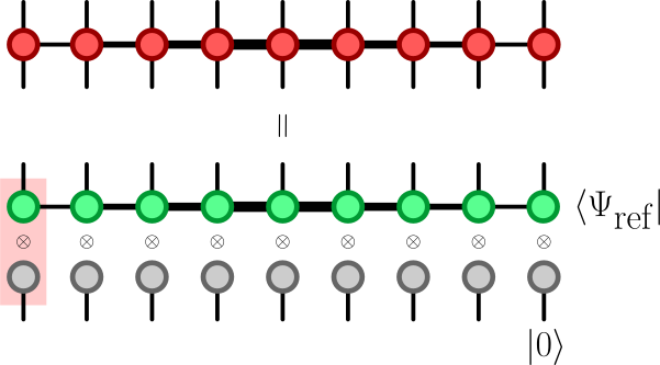
With the same cost function we can target also the problem of finding a good preparation circuit for some initial state in the form of an MPS. We just need to build \(\text{M}_{\mathrm{ref}}\) to represent the transition from an empty quantum register into the target MPS \(|0 \rangle^{\otimes L} \langle \Psi_{\mathrm{ref}} |\).

Note that in this case, the the cost function will unfold into a square tensor network with open boundary conditions, since the outer product used to build the reference MPO is just an encoding of the tensors.

# We pick a target state: the ground state of some local spin Hamiltonian in MPS form
ham_NNIM_mpo = ham_NNIM.to_mpo()
dmrg = DMRG2(ham_NNIM_mpo)
dmrg.solve(max_sweeps=16, bond_dims=64, verbosity=1, cutoffs=1e-12)
GS = dmrg.state

# We build the transition MPO from the empty register to the target MPS
GS_mpo = state_preparation_mpo(state_mps=GS)

# We feed the new reference MPO into the same routine as above
n_sweeps_max = 1000
rtol = 1e-6
list_depths = [1, 2, 3, 4]
for depth in list_depths:
    cost_tn_closed = init_cost_tn(
        ref_mpo=GS_mpo,
        depth=depth,
        param_scaling=1e-1,
        closed=True,
        seed=37,
    )

    dict_transf = find_transfer_structure(n_qubits=L, cost_tn=cost_tn_closed)

    dict_contr_envs = build_first_sweep(
        n_qubits=L, cost_tn=cost_tn_closed, dict_transf=dict_transf, drop_tags=True
    )
    print(f"Best overlap for depth {depth}:")
    opt_cost_tn, opt_dict_contr_envs = optimize_single_gate_update(
        n_qubits=L,
        cost_tn=cost_tn_closed,
        rtol=rtol,
        n_sweeps_max=n_sweeps_max,
        dict_transf=dict_transf,
        dict_contr_envs=dict_contr_envs,
    )

1, R, max_bond=(8/64), cutoff:1e-12

Energy: -4.432487024515108 ... not converged.

2, R, max_bond=(16/64), cutoff:1e-12

Energy: -4.43347172902142 ... not converged.

3, R, max_bond=(21/64), cutoff:1e-12

Energy: -4.433496252713884 ... converged!

Best overlap for depth 1:

Best overlap for depth 2:

Best overlap for depth 3:

Best overlap for depth 4: