10. Variational Circuit Preparation

10.1. Approximate ground states via tensor-network circuit optimization

We show how to represent an approximate ground state of an Hamiltonian expressed as Matrix-Product-Operator (MPO) as (i) a Matrix-Product-State (MPS), and as (ii) the wavefunction associated with a quantum circuit of finite depth. This reproduces (to some extent) the work of R. Haghshenas et al., Variational Power of Quantum Circuit Tensor Networks, Phys. Rev. X 12, 011047 (2022). This can be used to prepare an initial state for Quantum Phase Estimation (arxiv:2409.11748).

We also used some syntax and advice from the Tensor Network Training of Quantum Circuits example in \(\texttt{quimb}\)’s documentation.

import os

os.environ["OPENBLAS_NUM_THREADS"] = "1"
os.environ["JAX_ENABLE_X64"] = "True"

import autoray
import matplotlib.pyplot as plt
import numpy as np
import quimb.tensor as qtn

from qpe_toolbox.circuit import ansatz_circuit
from qpe_toolbox.estimation import qpe_sample, set_search_window
from qpe_toolbox.hamiltonian import heisenberg_hamiltonian

plt.rcParams.update({"font.size": 12})

opt = "auto-hq"

10.2. State preparation

10.2.1. The DMRG algorithm to find an MPS ground state

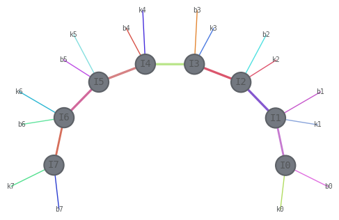
We first define our model Hamiltonian (Heisenberg chain) on \(n=8\) qubits. We know that its ground state can be approximated as a MPS. We use first the DMRG algorithm as a black box to have a reference energy (using a very large bond dimension 100 to have essentially the exact GS energy)

n_qubits = 8
hamilt = heisenberg_hamiltonian(n_qubits)
hamilt_mpo = hamilt.to_mpo()
hamilt_mpo.draw(
    show_tags=True, show_inds=True, edge_scale=1, layout="kamada_kawai", edge_color=True
)

dmrg = qtn.DMRG2(hamilt_mpo, bond_dims=[10, 20, 40, 100], cutoffs=1e-13)
dmrg.solve(tol=1e-6, verbosity=1)
dmrg_energy = np.real(dmrg.energy)
print("DMRG reference energy:", dmrg_energy)

1, R, max_bond=(10/10), cutoff:1e-13

Energy: (-3.374931217799727+0j) ... not converged.

2, R, max_bond=(10/20), cutoff:1e-13

Energy: (-3.3749325986878667+1.1102230246251565e-16j) ... not converged.

3, R, max_bond=(16/40), cutoff:1e-13

Energy: (-3.3749325986878818-3.3306690738754696e-16j) ... converged!

DMRG reference energy: -3.3749325986878818

10.2.2. MPS search via tensor-network differentiation

Let us now write a custom optimizer to find the ground state MPS, effectively performing the same task as in DMRG. The goal is simply to warm up for the circuit optimization that comes later.

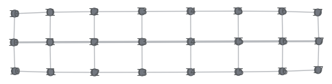
When one optimizes the energy \(H\) with respect to a variational wave function, we need first to be able to evaluate \(\braket{\psi|H|\psi}\) as a tensor contraction

psi = qtn.MPS_rand_state(n_qubits, bond_dim=2)
psiH = psi.H
psi.align_(hamilt_mpo, psiH)
energy_tn = psiH & hamilt_mpo & psi
print("Contracted energy:", energy_tn.contract(all, optimize=opt))
energy_tn.draw()

Contracted energy: (-0.7850974773699702+0j)

Now we can define a loss function, the energy, to be optimized w.r.t each tensor that makes the MPS \(\ket{\psi}\). We use \(\texttt{jax}\) as automatic differentiation tools to evaluate the gradients.

def loss(psi, mpo):
    psiH = psi.H
    norm_tn = psiH & psi
    psi.align_(mpo, psiH)
    energy_tn = psiH & mpo & psi
    energy = autoray.do("real", energy_tn.contract(all, optimize=opt))
    norm = autoray.do("real", norm_tn.contract(all, optimize=opt))
    return energy / norm


def myoptimizer(chi, mpo):
    psi = qtn.MPS_rand_state(n_qubits, bond_dim=chi)
    return qtn.TNOptimizer(
        psi,  # the tensor network we want to optimize
        loss,  # the function we want to minimize
        loss_constants={"mpo": mpo},
        autodiff_backend="jax",  # use 'autograd' for non-compiled optimization
        optimizer="L-BFGS-B",  # the optimization algorithm
    )

Let us optimize for a first bond dimension \(\chi=4\). This is already extremely fast and accurate.

tn_opt = myoptimizer(4, hamilt_mpo)
psi_opt = tn_opt.optimize(n=200)
print("Optimized energy ", tn_opt.loss)
print("Exact energy ", dmrg_energy)

Optimized energy  -3.371801709452784
Exact energy  -3.3749325986878818

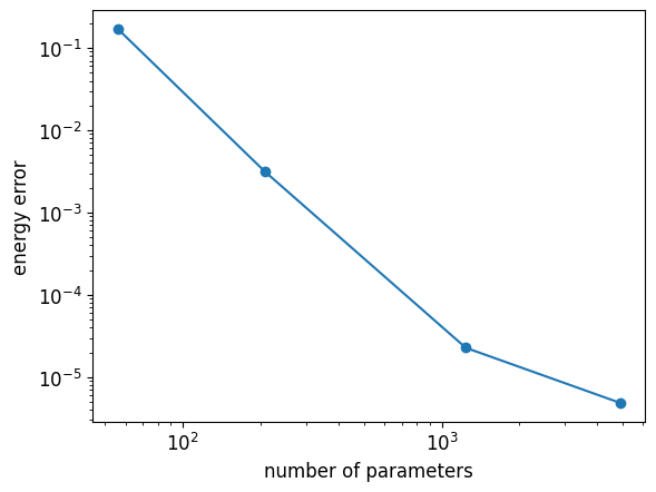
Let us be more quantitative by relating the energy estimation to the number of variational parameters \(d=2((n-2)\chi^2+2\chi)\) of an MPS, for various \(\chi\)

bond_dimensions = [2, 4, 10, 20]
n_values = len(bond_dimensions)
n_parameters = np.zeros(n_values)
optimized_energies = np.zeros(n_values)
for i in range(n_values):
    tn_opt = myoptimizer(bond_dimensions[i], hamilt_mpo)
    psi_opt = tn_opt.optimize(n=200)
    n_parameters[i] = tn_opt.d
    optimized_energies[i] = tn_opt.loss

plt.loglog(n_parameters, optimized_energies - dmrg_energy, "-o")
plt.xlabel("number of parameters")
plt.ylabel("energy error");

10.2.3. Finding a quantum circuit directly

MPS are good candidates for the initial state of the QPE algorithm because they can be prepared efficiently in a quantum computer. One possibility would be to find variationally the circuit that best approximates an MPS (see e.g. this recent proposal). Here, we take a shortcut, and directly find the circuit whose associated wavefunction minimizes the energy, in the spirit of R. Haghshenas et al., Variational Power of Quantum Circuit Tensor Networks. One practical advantage is that we may have less parameters to optimize using parametrized circuits compared to dense-tensors-based MPS.

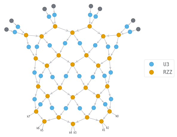
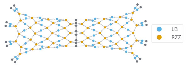
We consider finite-depth quantum circuits made of parametrized \(U_3\) single qubit rotations and \(R_{ZZ}\) two qubit gates.

Let us visualize the circuit wavefunction, and the tensor network contraction associated with the estimation of the energy.

depth = 4
circ = ansatz_circuit(n_qubits, depth)
psi = circ.psi
psi.draw(color=["U3", "RZZ"], show_inds=True)
psiH = psi.H
psi.align_(hamilt_mpo, psiH)
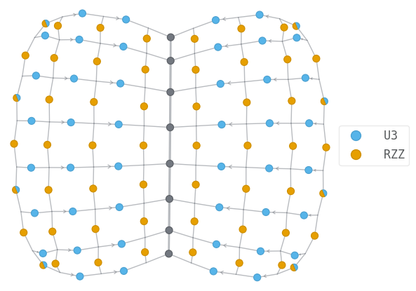
energy_tn = psiH & hamilt_mpo & psi
print(len(energy_tn.tensors))
energy_tn.draw(color=["U3", "RZZ"], show_inds=True)
simplified_tn = energy_tn.full_simplify()
print(len(simplified_tn.tensors))
simplified_tn.draw(color=["U3", "RZZ"], show_inds=True)

144

108

We can then define our optimizer on the angles that parametrize the gates.

def loss_circ(circ, mpo):
    psi = circ.psi
    psiH = psi.H
    norm_tn = psiH & psi
    psi.align_(mpo, psiH)
    energy_tn = psiH & mpo & psi
    energy = autoray.do("real", energy_tn.contract(all, optimize=opt))
    norm = autoray.do("real", norm_tn.contract(all, optimize=opt))
    return energy / norm


def make_circuit_optimizer(circ, mpo):
    return qtn.TNOptimizer(
        circ,  # the tensor network we want to optimize
        loss_circ,  # the function we want to minimize
        loss_constants={"mpo": mpo},  # supply U to the loss function as a constant TN
        autodiff_backend="jax",  # use 'autograd' for non-compiled optimization
        optimizer="L-BFGS-B",
    )

Let us make a first test. Since the contraction is a bit more involved than for straightforward MPS optimization, the simulation becomes a bit more tedious.

depth = 4
circ = ansatz_circuit(n_qubits, depth)
circ_optimizer = make_circuit_optimizer(circ, hamilt_mpo)
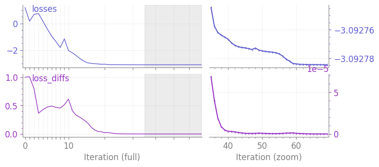
optimal_circuit = circ_optimizer.optimize(n=100)
print("Optimized energy ", circ_optimizer.loss)
print("Exact energy ", dmrg_energy)
circ_optimizer.plot();

Optimized energy  -3.191441136862914
Exact energy  -3.3749325986878818

It can be also interesting to optimize a circuit of large depth using the optimized parameters from a circuit of smaller depth. However as shown below, we don’t observe an improvement. So we will not use that in the following.

# optimize a shallow circuit
circ = ansatz_circuit(n_qubits, 2)
circ_optimizer = make_circuit_optimizer(circ, hamilt_mpo)
optimal_circuit = circ_optimizer.optimize(n=100)

# initialize a deeper circuit with previously optimized parameters
circ = ansatz_circuit(n_qubits, 4, param_scaling=1e-4)
circ.set_params(optimal_circuit.get_params())

# optimize the deeper circuit
circ_optimizer = make_circuit_optimizer(circ, hamilt_mpo)
optimal_circuit = circ_optimizer.optimize(n=100)
print("Optimized energy ", circ_optimizer.loss)
print("Exact energy ", dmrg_energy)

Optimized energy  -3.0615528098434437
Exact energy  -3.3749325986878818

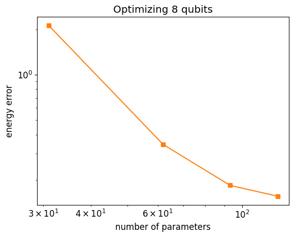
Let us analyze how things improve increasing the depth

max_depth = 4
depths = np.arange(1, max_depth + 1)
n_values = len(depths)
depth_parameters = np.zeros(n_values)
depth_energies = np.zeros(n_values)
for i in range(n_values):
    circ = ansatz_circuit(n_qubits, depths[i])
    circ_optimizer = make_circuit_optimizer(circ, hamilt_mpo)
    optimal_circuit = circ_optimizer.optimize(n=100)
    depth_parameters[i] = circ_optimizer.d
    depth_energies[i] = circ_optimizer.loss
    print("Depth ", depths[i])
    print("Current energy ", depth_energies[i])

Depth  1
Current energy  -1.2499999999880975

Depth  2
Current energy  -3.03077640499415

Depth  3
Current energy  -3.2152133183266898

Depth  4
Current energy  -3.260072334394258

plt.loglog(depth_parameters, depth_energies - dmrg_energy, "-s", color="tab:orange")
plt.xlabel("number of parameters")
plt.ylabel("energy error")
plt.title(f"Optimizing {n_qubits} qubits");

psi_exact = dmrg.state
overlap = (psi_exact.H & optimal_circuit.psi).contract()
print("fidelity ", abs(overlap) ** 2)

fidelity  0.9170002040282711

10.3. Quantum Phase Estimation

Let us know use a guess state the circuit optimization to initialize the QPE algorithm. For simplicity we will take a Hamiltonian defined on \(n=4\) qubits.

n_qubits = 4
hamilt = heisenberg_hamiltonian(n_qubits)
hamilt_mpo = hamilt.to_mpo()

dmrg = qtn.DMRG2(hamilt_mpo, bond_dims=[10, 20, 40, 100], cutoffs=1e-13)
dmrg.solve(tol=1e-6, verbosity=1)
dmrg_energy = np.real(dmrg.energy)
psi_exact = dmrg.state

print("\nStored reference energy ", dmrg_energy)

1, R, max_bond=(10/10), cutoff:1e-13

Energy: (-1.616025403784439-8.326672684688674e-17j) ... not converged.

2, R, max_bond=(4/20), cutoff:1e-13

Energy: (-1.61602540378444+5.551115123125783e-17j) ... converged!

Stored reference energy  -1.61602540378444

We take the shallowest circuit

depth = 1
circ = ansatz_circuit(n_qubits, depth)
circ_optimizer = make_circuit_optimizer(circ, hamilt_mpo)
optimal_circuit = circ_optimizer.optimize(n=100)

print("Optimized energy ", circ_optimizer.loss)
print("Exact energy ", dmrg_energy)

Optimized energy  -0.49999999996946454
Exact energy  -1.61602540378444

With this depth, we should be able to reach around 30% fidelity. If it isn’t the case, try to rerun the optimization

overlap = (psi_exact.H & optimal_circuit.psi).contract()
fidelity = abs(overlap) ** 2
print("fidelity ", fidelity)

fidelity  0.3110042339501942

Running QPE on a state with 30% overlap should increase the fidelity. Let us initialize a circuit with a physical register and a phase register. We take \(m=3\) phase qubits.

n_phase_qubits = 3

# circuit from optimized gates
circ_qpe = qtn.CircuitMPS(n_phase_qubits + n_qubits)

for gate in optimal_circuit.gates:
    label, params, qubits = gate.label, gate.params, gate.qubits
    qubits = tuple(qb + n_phase_qubits for qb in qubits)
    circ_qpe.apply_gate(label, *params, *qubits)

Set QPE parameters: first define the size of the search interval \(\Delta\) which sets the evolution time \(t\)

E_target = circ_optimizer.loss
size_interval = 3
E_const, Emax, evolution_time, global_phase = set_search_window(
    hamilt, E_target, size_interval
)

and the Trotter parameters

trotter_order = 2
n_steps = 4
dt = evolution_time / n_steps

then run textbook QPE (this can take a minute or two). Since n_qubits is small, for faster execution you can always use exact time evolution instead of a Trotterization.

%%time
traces, res = qpe_sample(
    hamilt, circ_qpe, evolution_time, dt, global_phase, trotter_order=trotter_order
)

CPU times: user 45.7 s, sys: 723 ms, total: 46.4 s
Wall time: 44.1 s

NB: the energy minimum can be \(< E_{\rm exact}\) when \(E_{\rm target} - \Delta/2 < E_{\rm exact}\). We only consider the bitstrings with probability \(> 4/\pi^2 F\) where \(F = |\langle{\psi}|\psi_{\rm exact}\rangle|^2\). The \(4/\pi^2\) factor gives a lower bound on the QPE success probability depending on the initial overlap as explained in the Textbook QPE example.

NB: in practice one will not have access to the overlap. An approximation of the fidelity is sufficient. The following quantity can be used as a proxy, see arxiv:2306.02620:

\[ F \approx \exp\Big(- \frac{(E-E_0)^2}{2\sigma^2}\Big ),\]

where \(\sigma = \langle H^2 \rangle - E^2\) is the energy variance on guess state \(\ket{\psi}\), and \(E_0\) is an estimate of the exact ground state energy that doesn’t need to be very accurate.

k_probs_list = sorted(enumerate(np.ravel(res)), key=lambda x: x[1], reverse=True)

kmin = 2 ** (n_phase_qubits - 1)
prob_min = 0
emin = E_target
energies = []

for k, prob in k_probs_list:
    energy = E_target + size_interval * (1 / 2 - k / 2**n_phase_qubits)
    energies.append(energy)
    if energy < emin and prob > fidelity * 4 / np.pi**2:
        emin = energy
        kmin = k
        prob_min = prob

print(f"Most probable energy = {energies[0]:.5f} w prob = {k_probs_list[0][1]:.5f}")
print(f"First 5 energies = {np.round(energies[:5], 5)}")
print(f'Minimal "significant" energy = {emin:.5f} with probability {prob_min:.5f}')
print(
    f"error = {abs(dmrg_energy - emin):.5f} (theoretical error bound = {size_interval / 2**n_phase_qubits:.5f})"
)

Most probable energy = -0.12500 w prob = 0.33323
First 5 energies = [-0.125 -1.625  0.625 -0.5    0.25 ]
Minimal "significant" energy = -1.62500 with probability 0.32249
error = 0.00897 (theoretical error bound = 0.37500)

When the GS energy is measured, the physical register contains the GS wavefunction. We thus project the phase register of the final circuit wavefunction on the previously found bitstring that gives the minimal energy while satisfying the probability criterion

psi_final = traces["circuit"].psi
# change psi_final.backend from 'jax' to numpy as a workaround for
# https://github.com/jcmgray/quimb/issues/340
psi_final.apply_to_arrays(np.asarray)

bin_kmin = f"{kmin:b}".zfill(n_phase_qubits)
for i in range(n_phase_qubits):
    psi_final.measure_(0, outcome=int(bin_kmin[i]), remove=True)

The fidelity should improve

overlap_qpe = psi_final.overlap(psi_exact)
fidelity_qpe = abs(overlap_qpe) ** 2
print(f"Fidelity before QPE = {fidelity:.5f}")
print(f"Fidelity after QPE = {fidelity_qpe:.5f}")

Fidelity before QPE = 0.31100
Fidelity after QPE = 0.96258

We observe that even with a moderate overlap, Quantum Phase Estimation projects on the ground state. As an exercise, you can try to reproduce the following figure:

it shows the infidelity as a function of circuit depth (orange curve) or bond dimension (blue curve) for a guess state prepared with either circuit optimization or DMRG. The colored stars then show how the fidelity quickly improves (error drops to \(\sim 10^{-5}\)) when running QPE with even a few phase qubits upon the trial state from circuit optimization.