8. quimb - qiskit MPS benchmark

Recent studies comparing different quantum backends, like the one collected in feniqs_lite, have pointed out that \(\texttt{qiskit-aer}\) may be one of the fastest options to execute and sample a quantum circuit with classical resources, thanks to its underlying Rust/C++ implementation. Nevertheless, in a simple comparative study, we detect that this advantage depends strongly on the underlying circuit architecture when compared with \(\texttt{quimb}\).

In this example, we explore the contraction and sampling times for two types of circuits: brickwork and random entangling patterns. Carrying out several simulations with the respective MPS classes in \(\texttt{qiskit-aer}\) and \(\texttt{quimb}\), we find that \(\texttt{quimb}\) becomes faster than \(\texttt{qiskit-aer}\) for deep enough circuits constituted by long-range gates. The data used in this study were computed on a laptop using a single CPU thread and are loaded from the accompanying JSON files.

import json
import os
from collections import Counter

os.environ["NUMBA_NUM_THREADS"] = "1"
os.environ["OMP_NUM_THREADS"] = "1"
os.environ["MKL_NUM_THREADS"] = "1"

import matplotlib.pyplot as plt
import numpy as np
from qiskit.visualization import plot_histogram
from qiskit_aer import AerSimulator

from qpe_toolbox.circuit import (
    deserialize_to_qiskit_QuantumCircuit,
    deserialize_to_quimb_Circuit,
    deserialize_to_quimb_CircuitMPS,
    draw_layered_circuit,
    generate_rand_circuit,
    serialize_from_quimb_Circuit,
)

def plot_errorbar(ax, x, y, yerr, mfc, *, fmt="o", label=None):
    return ax.errorbar(
        x,
        y,
        yerr,
        fmt=fmt,
        mfc=mfc,
        label=label,
        markersize=6,
        markeredgecolor="k",
        color="black",
        ecolor="black",
        elinewidth=0.5,
        capsize=6,
        capthick=0.5,
    )

8.1. Circuit instances

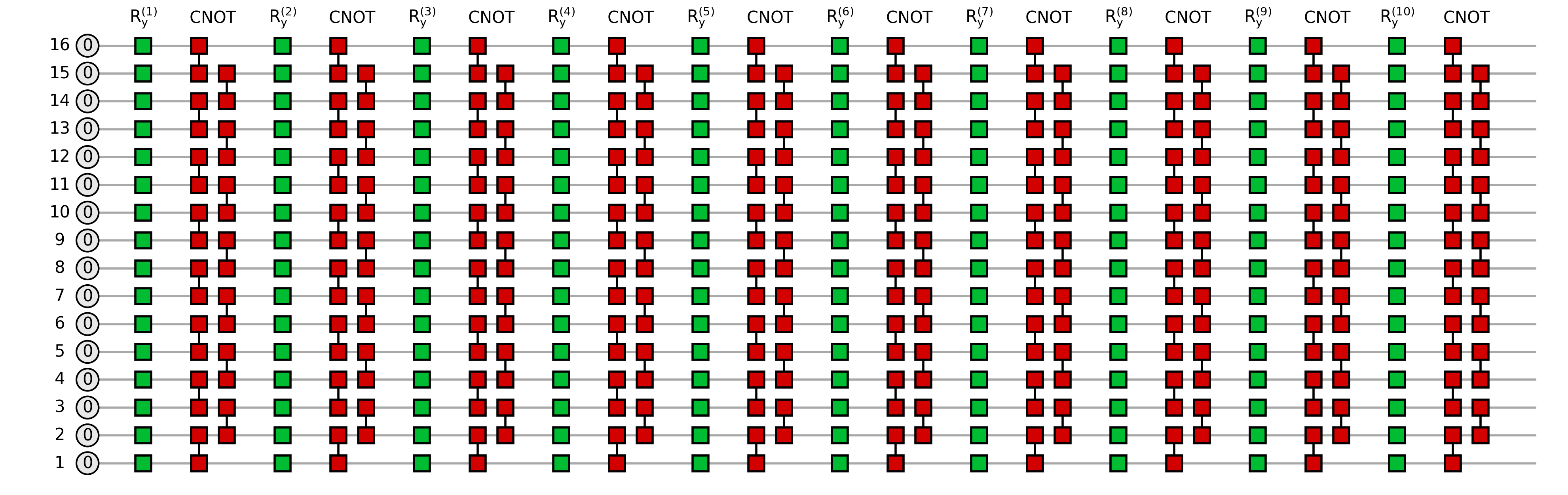
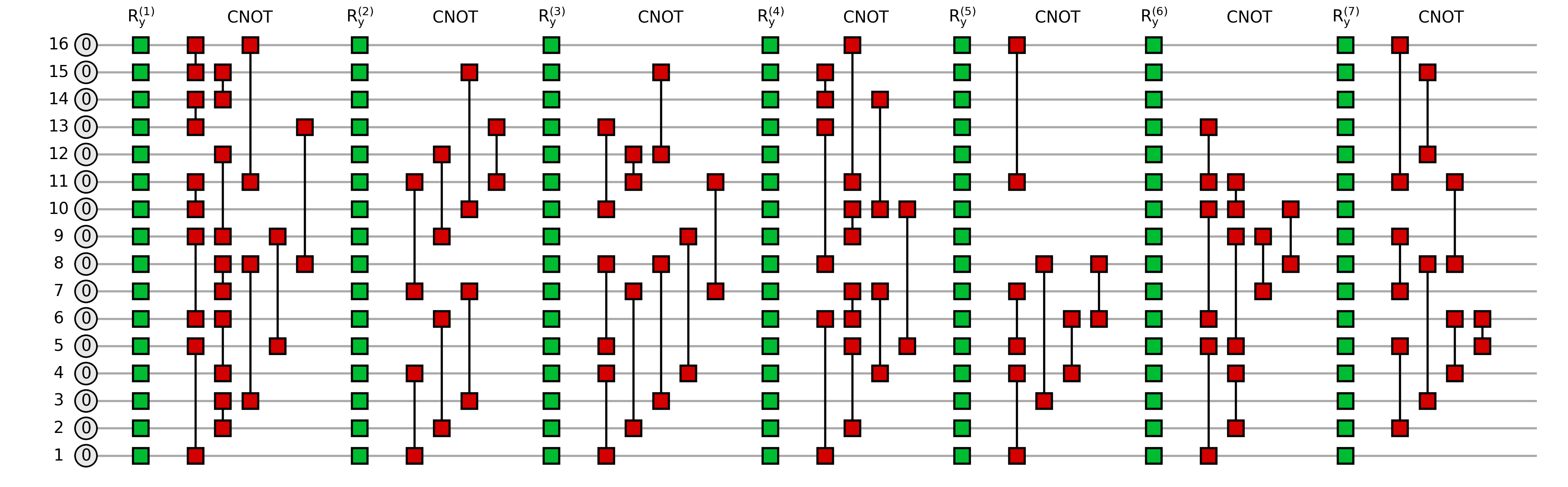
Let us visualize the smallest instances of circuits that explored throughout this example:

circuit_types = ("brick", "rand")
circuit_data = {}
for ctype in circuit_types:
    with open("precomputed_data/" + ctype + "_circ_perfo.json") as fin:
        circuit_data[ctype] = json.load(fin)

for ctype in circuit_types:
    circ = deserialize_to_quimb_Circuit(circuit_data[ctype][ctype + "_16"])
    depth = max([gate.round for gate in circ.gates]) + 1
    fig = draw_layered_circuit(
        circ,
        list_names=[
            r"$0$",
            [f"$\\mathrm{{R_y^{{({j})}} }}$" for j in range(1, depth + 1)],
            [r"$\mathrm{CNOT}$"] * depth,
        ],
        max_depth=depth,
    )

The next cell contains a short code example demonstrating how we compare simulation timings:

(1) we create or load already existing circuits with the functions introduced in building_circuits,

(2) we run simulations (circuit execution + sampling) and access the times and samples,

(3) we compare the results for both backends.

The following code is also a sample of how we obtained the pre-computed data (note that we fixed the number of threads to 1):

# Create small circuit
depth = 3
circ_quimb = generate_rand_circuit(
    n_qubits=5,
    depth=depth,
    one_qubit_gate_label="rx",
    two_qubit_gate_label="cx",
    two_qubit_gate_range=4,
    two_qubit_gate_prob=0.5,
)

# Recast it into the right classes
circ_dict = serialize_from_quimb_Circuit(circ_quimb)
circ_quimb = deserialize_to_quimb_CircuitMPS(
    full_gate_dict=circ_dict, max_bond=2**depth, cutoff=10e-8
)
circ_qiskit = deserialize_to_qiskit_QuantumCircuit(circ_dict, measure=True)

num_samples = 10**4  # pick the number of samples
# Run qiskit
simulator = AerSimulator(
    method="matrix_product_state",
    matrix_product_state_max_bond_dimension=2**depth,
    matrix_product_state_truncation_threshold=10e-8,
    seed_simulator=1,
)
result = simulator.run(circ_qiskit, shots=num_samples).result()
# qiskit inverts the layout order
counts_qiskit = Counter({k[::-1]: v for k, v in result.get_counts().items()})

# Run quimb
counts_quimb = Counter(circ_quimb.sample(C=num_samples, seed=42))

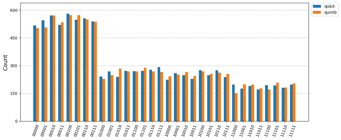
We can compare the bitstring histogram from both simulations as a sanity check:

plot_histogram(
    [counts_qiskit, counts_quimb],
    legend=["qiskit", "quimb"],
    bar_labels=False,
    figsize=(12, 5),
)

8.2. Dependence of contraction and sampling times for quimb

In the following we present a non-exhaustive study of the dependence of the MPS (layer-by-layer) contraction time \(t_{\mathrm{contr}}\) and sampling \(t_{\mathrm{sampl}}\) in \(\texttt{quimb}\). We will seek the trend of these times as the number of qubits n_qubits (length of the MPS) and depth rise; note that the depth of the circuit upper bounds the bond dimension \(\chi\) of the fully contracted MPS as \(\chi \leq 2^{\rm depth}\).

We will compare the results for both types of quantum circuit instances introduced above. Since these classes of circuits are both random (in the sense that the parametrization of the single body gates is random), a thorough study would require averaging over circuit architectures and parametrizations. Such a study is beyond the scope of this example; we will actually observe that without averaging out this randomness we can extract solid comparisons.

The conditions of the simulations include:

• A maximum bond dimension max_bond \(\chi=2^{\rm depth}\), such that the simulation should not introduce any norm truncation due to bond dimension capping.

• A cutoff parameter, set to \(\varepsilon=10^{-10}\); this cutoff controls the tail of singular values that is cut out after a local gate application.

A more natural prescription for the study than the one chosen here would be to set a maximum accumulated error in the norm \(\varepsilon_{\mathrm{total}}\), and study the growth of \(t_{\mathrm{contr}}\), \(t_{\mathrm{sampl}}\) and \(\chi\) for that fixed threshold in n_qubits and \(\chi\). We avoid this prescription due to the difficulty of fixing the maximum error across different backends.

8.2.1. Dependence in the number of qubits

In the following plot we present our results in two columns: the left for brickwall circuits, and the right for random circuits. The chosen depths are depth=1, 3, 5, and the \(\texttt{quimb}\) class \(\texttt{PermMPS}\) is also used for random circuits with depth=1:

mycolors = ("tab:red", "tab:orange", "tab:olive", "tab:purple", "tab:pink", "tab:cyan")
cases = ("quimb MPS contr", "quimb MPS sampl 1", "quimb MPS sampl 10")
cases_perm = ("quimb PermMPS contr", "quimb PermMPS sampl 1", "quimb PermMPS sampl 10")
dum = np.array([np.nan])
circuit_sizes = 2 ** np.arange(4, 9)
x_lines = np.linspace(circuit_sizes[0] / 2, circuit_sizes[-1] * 2)
ylims = ((5e-4, 1.0), (1e-3, 1.0), (1e-3, 10.0))
fig, axes = plt.subplots(3, 2, sharex=True, figsize=(5 * 2, 5 * 3 / 1.61))
for idx, ax in np.ndenumerate(axes):
    for instance in circuit_data[circuit_types[idx[1]]].values():
        for i, c in enumerate(cases):
            values = instance[f"depth{2 * idx[0] + 1}"][c]
            plot_errorbar(
                ax, instance["n_qubits"], np.mean(values), np.std(values), mycolors[i]
            )
    ax.set_xlim(circuit_sizes[0] / 2, circuit_sizes[-1] * 2)
    ax.set_xscale("log", base=2)
    ax.set_yscale("log")
    ax.set_xticks(circuit_sizes)
    ax.get_xaxis().set_major_formatter(plt.ScalarFormatter())
    ax.grid(which="both", linestyle="-", linewidth=0.25, alpha=0.5)
    ax.set_ylim(ylims[idx[0]])
    for m in range(16):
        ax.plot(x_lines, 10 ** (m / 2) / 8e5 * x_lines, "-", color="grey", alpha=0.1)
for instance in circuit_data[circuit_types[1]].values():
    for i, c in enumerate(cases_perm):
        values = instance["depth1"][c]
        plot_errorbar(
            axes[0, 1],
            instance["n_qubits"] * 1.15,
            np.mean(values),
            np.std(values),
            mycolors[i + 3],
            fmt="s",
        )
for i in range(3):
    axes[i, 0].set_ylabel(rf"$\text{{depth}}={2 * i + 1}$")
    axes[i, 1].set_yticklabels([])
    plot_errorbar(axes[0, 1], dum, dum, dum, mycolors[i], label=cases[i][6:])
    plot_errorbar(
        axes[0, 1], dum, dum, dum, mycolors[i + 3], fmt="s", label=cases_perm[i][6:]
    )
axes[0, 0].set_title("brickwall circuits")
axes[0, 1].set_title("random circuits")
axes[0, 1].legend(loc="lower right", fontsize=8)
axes[2, 0].set_xlabel("number of qubits")
axes[2, 1].set_xlabel("number of qubits")
fig.text(0.04, 0.5, "wall-clock time", va="center", rotation="vertical", fontsize=16)
fig.tight_layout(rect=[0.05, 0.05, 1, 0.95])

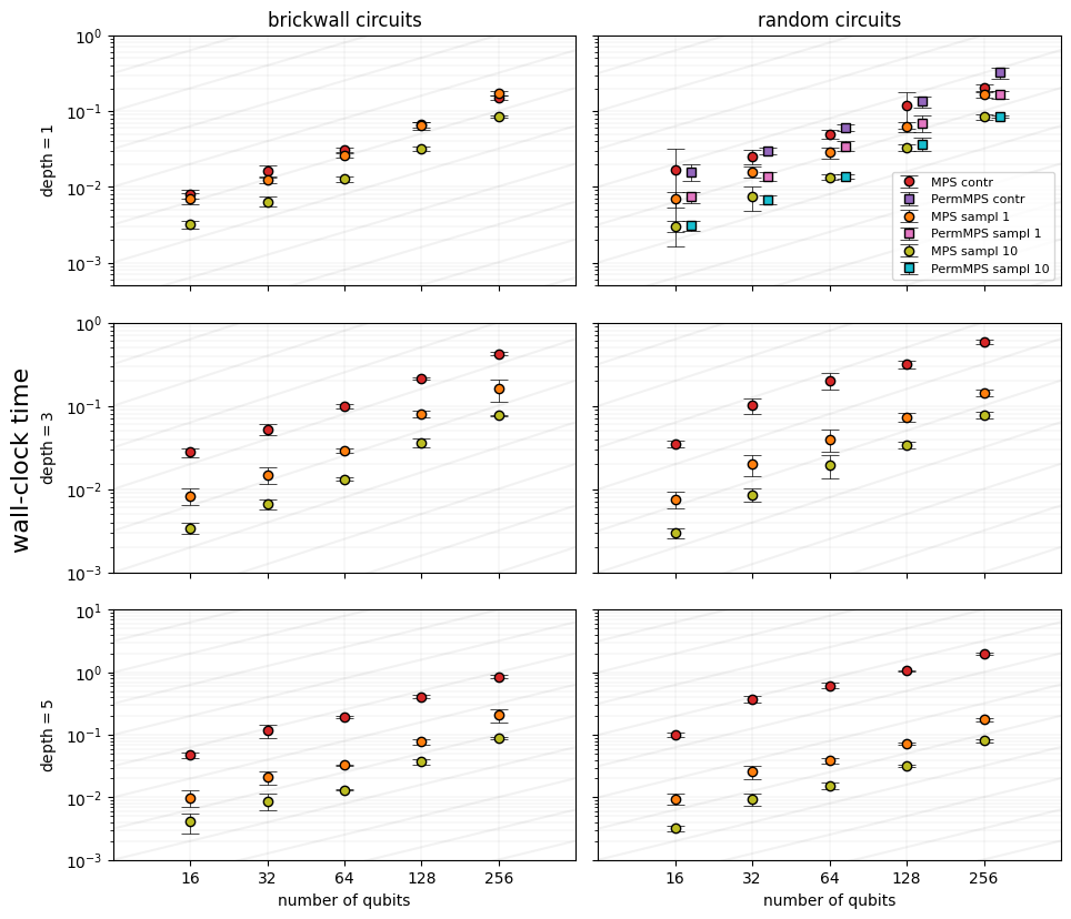
Both the contraction and sampling times vary linearly with the number of qubtis. Indeed the circuit classes treated here involve a number of gates proportional to the number of qubits in the register, therefore the circuit contraction process repeats the gate application procedure an amount times that is \(\propto n_{\rm qubits}\). This behavior is reflected by the scaling of the red markers. To highlight the scaling, a set of parallel power-law lines \(\propto n_{\rm qubits}\) are added to the grid as a guide to the eye.

Conversely, the sampling requires finding the probability marginals for different outcomes by setting the \(n_{\rm qubits}\) bitstring. Therefore, the scaling of sampling times with the number of qubits is also \(\propto n_{\rm qubits}\).

Note though, that it is not the same to sample a single bitstring or 10 bitstrings in one go: the sample method from \(\texttt{quimb}\) caches the marginal distributions between calls; this means that sampling more and more bitstrings gets everso faster than a single bitstring. This effect is reflected by the gap between the orange markers (1 sample) and the yellow markers (10 samples): the later indicate the average sampling time for drawing 10 bitstrings (thus we are timing sample(C=10)/10 rather than sample(C=1)).

The former discussion was fully dedicated to the CircuitMPS class from \(\texttt{quimb}\). Nevertheless, there exists another MPS class that tries to leverage the non-locality of long-range circuits: PermMPS. The goal of this class can be understood by diving a bit into the procedure for applying a long-range gate: it requires permuting the two involved qubits through the 1-dimensional layout until they are nearest-neighbors, followed by the local application of the two-body gate. While CircuitMPS would restore the initial layout after the gate application, PermMPS leaves this new layout and tracks the intermediate trajectories of the qubits. Obviously, this class may yield advantageous wall-clock time measures when the number of gates is sparse. Opposed to that, our circuit instances are not sparse enough to detect a clear advantage. This can be seen for depth=1 in the right column (random entangling pattern). Despite these results, we expect that a study with varying ent_prob and ent_range in the function generate_rand_circuit would define a regime of dominance of PermMPS over CircuitMPS for sparse circuits (low ent_prob, medium-low ent_range).

8.2.2. Dependence in the bond dimension

In the following plot we present our results in two columns: the left for brickwall circuits, and the right for random circuits. The chosen circiuit sizes are \(n_{\rm qubits} \in \{64, 128, 256\}\):

x_range = np.linspace(1, 256)
n_qubits_values = (64, 128, 256)
depths = range(1, 8)
ylims = ((1e-2, 5.0), (1e-2, 1e2), (1e-2, 1.0), (1e-2, 5.0))
mycolors = ("tab:blue", "tab:orange", "tab:green")
fig, axes = plt.subplots(2, 2, sharex=True, figsize=(10, 5 * 2 / 1.61))
for iN, n_qubits in enumerate(n_qubits_values):
    plot_errorbar(
        axes[0, 0], dum, dum, dum, mycolors[iN], label=rf"n_qubits={n_qubits}"
    )
    for j, ctype in enumerate(circuit_types):
        for depth in depths:
            data = circuit_data[ctype][f"{ctype}_{n_qubits}"]
            bond_dim = data[f"depth{depth}"]["quimb MPS bondim"]
            values = (
                data[f"depth{depth}"]["quimb MPS contr"],
                data[f"depth{depth}"]["quimb MPS sampl 1"],
            )
            for k, ax in enumerate(axes[:, j]):
                plot_errorbar(
                    ax,
                    bond_dim,
                    np.mean(values[k]),
                    np.std(values[k]),
                    mycolors[iN],
                )
                if depth == max(depths):
                    y = x_range ** (3 - k) * np.mean(values[k]) / bond_dim ** (3 - k)
                    ax.plot(x_range, y, "-", color="grey", alpha=0.1)
axes = axes.flatten()
for i, ax in enumerate(axes):
    ax.set_xlim(x_range[0], x_range[-1])
    ax.set_xticks(2 ** np.arange(2, 8))
    ax.set_xscale("log", base=2)
    if i > 1:
        ax.set_xlabel("bond dimension")
    ax.get_xaxis().set_major_formatter(plt.FuncFormatter(lambda x, _: f"{int(x)}"))
    ax.set_ylim(ylims[i])
    ax.set_yscale("log")
    ax.grid(which="both", linestyle="-", linewidth=0.25, alpha=0.5)
axes[0].set_title("brickwall circuits")
axes[0].set_ylabel("contraction")
axes[1].set_title("random circuits")
axes[2].set_ylabel("sampling")
axes[0].legend(loc="lower right", fontsize=8)
fig.text(0.04, 0.5, "wall-clock time", va="center", rotation="vertical", fontsize=16)
fig.tight_layout(rect=[0.05, 0.05, 1, 0.95])

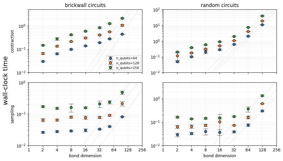
In order to understand scaling of the contraction and sampling times with the bond dimension we first need to recall which are the algorithmic expectations for each case.

The contraction procedure involves (as mentioned earlier) the application of a two-body gate onto a pair of local tensors on an MPS, which at a given depth may have a bond dimension \(\chi\leq 2^{\rm depth}\). The algorithmic cost for this contraction is \(\propto \chi^3\), as it can be easily computed by dimension arguments. This scaling only becomes visible for the largest bond dimensions in the right column for the random entangling pattern circuits, which at the same time saturate the bound between the circuit depth and the bond dimension: \(\chi=2^{\rm depth}\). As a guide to the eye, we have added the cubic power law that passes by the points with highest \(\chi\).

For the case of sampling a single bitstring, the scaling can be trickier: sampling a single bitstring requires constructing the diagonal of a reduced density matrix, which can be done with cost \(\propto \chi^2\) if we consider only contracting the bra and ket parts of the MPS around the sites where the bitstring outcome is to be fixed. This is actually the scaling observed in the lower row of results for all the intances (see quadratic power law in grey passing by the points with highest \(\chi\)); despite that, we want to note that before contracting the MPS bra and ket, the MPS must be canonicalized. If the cost of such a process was to be included within the sampling time, then the cost would scale as \(\propto \chi^3\), due to the cost of performing rank-revealing matrix decompositions.

8.3. Comparison between quimb and qiskit-aer

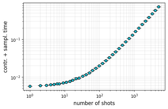
In the case of \(\texttt{qiskit-aer}\) backend, the contraction and sampling times cannot be easily split apart; this means that the simulator only returns \(t_{\mathrm{total}}(n_{\mathrm{sampl}})\), which is not necessarily equal to \(t_{\mathrm{total}}(n_{\mathrm{sampl}})=t_{\mathrm{contr}}+n_{\mathrm{sampl}}\cdot t_{\mathrm{sampl}}\). The simplest way to estimate \(t_{\mathrm{contr}}\) could be to repeat the simulation for a fixed circuit architecture and a list of \(n_{\mathrm{sampl}}\) values, and to deduce \(t_{\mathrm{contr}}\) and \(t_{\mathrm{sampl}}\) from a \(n_{\mathrm{sampl}}\to 0\) extrapolation. Nevertheless, when we explored this behavior for few instances, we found that there exist different regimes where the extrapolation would follow a particular scaling power law in \(n_{\mathrm{sampl}}\):

n_qubits = 32
num_samples = np.rint(np.logspace(np.log10(1), np.log10(5000), num=40)).astype(int)
num_repetitions = 5
depth = 3
qc = deserialize_to_qiskit_QuantumCircuit(
    circuit_data["brick"][f"brick_{n_qubits}"], max_depth=depth + 1, measure=True
)
dict_total_qiskit = {}
for shots in num_samples:
    batch_total_qiskit = np.empty(num_repetitions)
    for r in range(num_repetitions):
        simulator = AerSimulator(
            method="matrix_product_state",
            matrix_product_state_max_bond_dimension=2**depth,
            matrix_product_state_truncation_threshold=10e-8,
            mps_log_data=True,
        )
        result = simulator.run(qc, shots=shots).result()
        batch_total_qiskit[r] = result.time_taken

    dict_total_qiskit[shots] = {
        "mean": np.mean(batch_total_qiskit),
        "std": np.std(batch_total_qiskit),
    }

In the following plot we detect several regimes with different potential extrapolation slopes:

fig, ax = plt.subplots(1, 1, figsize=(6, 6 / 1.61))
for key, instance in dict_total_qiskit.items():
    plot_errorbar(ax, key, instance["mean"], instance["std"], "tab:cyan")
ax.set_ylabel("contr. + sampl. time", fontsize=12)
ax.set_xlabel("number of shots", fontsize=12)
ax.set_xscale("log")
ax.set_yscale("log")
ax.grid(which="both", linestyle="-", linewidth=0.25)

Therefore we restrain ourselves to compare the total wall-clock time for contracting the different circuits and sample 10 strings in both backends:

n_qubits_values = 2 ** np.arange(4, 9)
fig, axes = plt.subplots(3, 2, sharex=True, figsize=(5 * 2, 5 * 3 / 1.61))
for idx, ax in np.ndenumerate(axes):
    depth = idx[0] + 4
    for instance in circuit_data[circuit_types[idx[1]]].values():
        contr_quimb = np.asarray(instance[f"depth{depth}"]["quimb MPS contr"])
        sampl_quimb = np.asarray(instance[f"depth{depth}"]["quimb MPS sampl 10"])
        total_quimb = contr_quimb + sampl_quimb
        total_qiskit = np.asarray(instance[f"depth{depth}"]["qiskit total"])
        x = instance["n_qubits"]
        plot_errorbar(ax, x, np.mean(total_quimb), np.std(total_quimb), "tab:orange")
        plot_errorbar(ax, x, np.mean(total_qiskit), np.std(total_qiskit), "tab:cyan")

    ax.set_xlim(n_qubits_values[0] / 2, n_qubits_values[-1] * 2)
    ax.set_xscale("log", base=2)
    ax.set_yscale("log")
    ax.set_xticks(n_qubits_values)
    ax.get_xaxis().set_major_formatter(plt.ScalarFormatter())
    ax.grid(which="both", linestyle="-", linewidth=0.25)
    if idx[1] == 0:
        ax.set_ylabel(rf"$\text{{depth}}={depth}$")
    if idx[0] == 2:
        ax.set_xlabel("number of qubits")
plot_errorbar(axes[0, 0], dum, dum, dum, "tab:orange", label="quimb")
plot_errorbar(axes[0, 0], dum, dum, dum, "tab:cyan", label="qiskit=aer")
axes[0, 0].legend(loc="lower right", fontsize=12)
axes[0, 0].set_title("brickwall circuits", fontsize=12)
axes[0, 1].set_title("random circuits", fontsize=12)
fig.text(0.04, 0.5, "wall-clock time", va="center", rotation="vertical", fontsize=12)
fig.tight_layout(rect=[0.05, 0.05, 1, 0.95])

Interestingly, while for all sizes and depths of the chosen brickwall circuits \(\texttt{qiskit-aer}\) dominates with speedups of almost an order of magnitude, the same cannot be told for random circuits with long-range entangling gates. We observe that for deep enough instances (\({\rm depth}\geq 4\)), \(\texttt{qiskit-aer}\) and \(\texttt{quimb}\) already perform comparably; for the deepest random circuits explored here, \(\texttt{quimb}\) surpasses \(\texttt{qiskit-aer}\) by an order of magnitude.

8.4. Other strategies within quimb

Despite we already found some counterexamples to results like the ones gathered in feniqs_lite, we are well aware that \(\texttt{quimb}\) can offer even more by introducing more flexible quantum circuit classes (like Circuit) and methods suited for different architectures:

• sample : uses light-cone simplification and caching of the marginal distributions for chosen groupings of qubits.

• sample_gate_by_gate : achieves a cost for sampling similar to that of computing single amplitudes, but enlarges the amount of tensor networks to be contracted. This method was introduced in 2021.

• sample_chaotic : assumes that only subgroups of qubits are correlated, while the rest of the sampled bitstring results are essentially random. This strategy was successful at classically replicating one of the latest quantum advantage claims.