1. Building circuits

In this notebook we will explain step by step how to create, plot, record and load quantum circuits in \(\texttt{quimb}\) and \(\texttt{qiskit}\).

import json

import numpy as np
import quimb.tensor as qtn
from qiskit import QuantumCircuit
from qiskit.circuit.library import n_local
from qiskit.qasm2 import dumps
from qiskit_quimb import quimb_circuit

from qpe_toolbox.circuit import (
    deserialize_to_qiskit_QuantumCircuit,
    deserialize_to_quimb_Circuit,
    draw_layered_circuit,
    dump_quimb_Circuit_to_qasm,
    generate_brickwall_circuit,
    generate_rand_circuit,
    load_qasm_to_quimb_Circuit,
    serialize_from_quimb_Circuit,
)

1.1. Using \(\texttt{quimb}\)

1.1.1. Create custom circuits

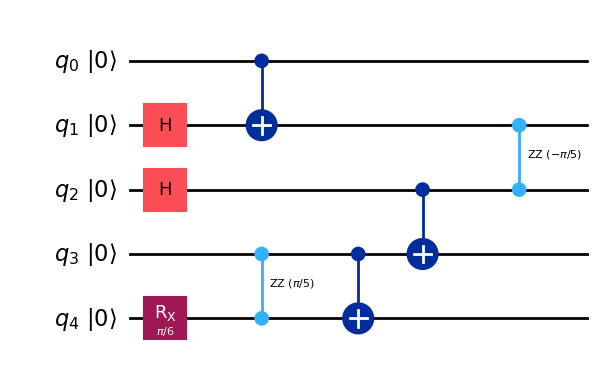
In the first place we need to know how wide our circuit is, i.e. specify the number of qubits on which the protocol will be executed. Once we know this, we can call the class Circuit to generate an empty instance. Once we have our empty instance, we will start appending the gates of interest, according to the quantum algorithm that we aim to execute. \(\texttt{quimb}\) includes a list of constant and parametrizable one- and two-qubit gates that can be used for gate-by-gate construction. For example:

rng = np.random.default_rng(42)
n_qubits = 5  # total number of qubits
circ = qtn.Circuit(n_qubits)  # instantiate the class, get an empty circuit

# Hadamard on the 2nd qubit and 0th layer
circ.apply_gate(gate_id="h", qubits=[1], gate_round=0)

circ.apply_gate(gate_id="h", qubits=[2], gate_round=0)

# 'Rx' with angle 'pi/6' on the 5th qubit and 0th layer
circ.apply_gate(gate_id="rx", params=[np.pi / 6], qubits=[4], gate_round=0)

# CNOT from 1st to 2nd qubits in the 1st layer
circ.apply_gate(gate_id="cx", qubits=[0, 1], gate_round=1)

# 'Rzz' with angle 'pi/5' between 4th to 5th qubits, 1st layer
circ.apply_gate(gate_id="rzz", params=[np.pi / 5], qubits=[3, 4], gate_round=1)

circ.apply_gate(gate_id="cx", qubits=[3, 4], gate_round=2)
circ.apply_gate(gate_id="cx", qubits=[2, 3], gate_round=3)
circ.apply_gate(gate_id="rzz", params=[-np.pi / 5], qubits=[1, 2], gate_round=4)

When applying each one of the gates, we added further information on the gate_round; this information can be used for multiple purposes, like visualization. \(\texttt{quimb}\) includes ‘pre-cooked’ recipes for well-known circuits like the QAOA Ansatz, such that they do not need to be rebuilt from scratch (see the list here ). We also provide some functions with simple brick-wall and random circuits, which are the main focus of our performance.py example:

# Build a circuit with random parameters and two-layer structure;
# one layer is a single-body rotation, and the other is
# an entangling two-body gate
brickwall_circuit = generate_brickwall_circuit(
    n_qubits=10,
    depth=4,
    one_qubit_gate_label="rx",
    two_qubit_gate_label="cnot",
    rng=rng,
)

# Same as before, but the entangling layer randomly picks pairs
# of qubits at a maximum distance `ent_range`
random_circuit = generate_rand_circuit(
    n_qubits=10,
    depth=4,
    one_qubit_gate_label="rx",
    two_qubit_gate_label="cnot",
    two_qubit_gate_range=3,
    two_qubit_gate_prob=0.33,
    rng=rng,
)

1.1.2. Plotting circuits

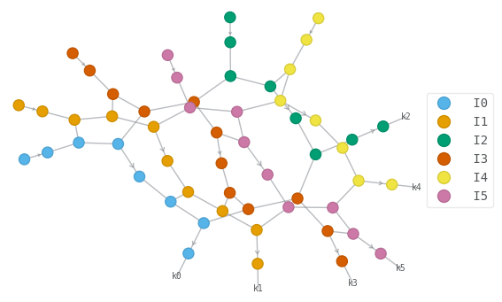
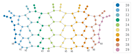
\(\texttt{quimb}\) includes visualization tools native from \(\texttt{networkx}\), specialized on graphs. Therefore, if the user is interested on seeing the circuit as a graph, this is the right plotting tool. As a short example, we present how \(\texttt{quimb}\) can automatically manage coloring by labels (gate type), index (qubit position) and round (depth in which the gate was applied) with graph layout:

# Indicate the set of tensors acting on particular qubits
brickwall_circuit.psi.draw(color=[f"I{i}" for i in range(brickwall_circuit.N)])

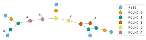
# Indicate the gate round
depth = max(gate.round for gate in circ.gates) + 1
circ.psi.draw(color=["PSI0"] + [f"ROUND_{i}" for i in range(depth)])

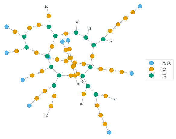
# Indicate different gates
random_circuit.psi.draw(color=["PSI0", "RX", "CX"], layout="kamada_kawai")

Nevertheless, to understand the details of large circuits with long-range gates, it is preferable to switch to matplotlib, as crossings of tensor legs in the network can be clarified using a fixed layout. To this end, we introduce draw_layered_circuit, which targets circuits composed of layers of single- and two-qubit rotations:

depth = max([gate.round for gate in random_circuit.gates]) + 1
fig = draw_layered_circuit(
    random_circuit,
    list_names=[
        r"$0$",
        [f"$\\mathrm{{R_x^{{({i})}} }}$" for i in range(1, depth + 1)],
        [r"$\mathrm{CNOT}$"] * depth,
    ],
    max_depth=depth,
)

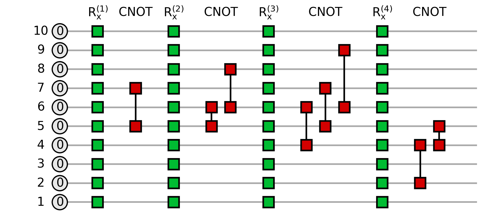
The rationale behind draw_layered_circuit is the very same as the schematic module of \(\texttt{quimb}\), but we chose to build it ourselves for better picture scaling.

1.1.3. Recording and loading circuits

We are also interested on saving our circuits for later use. For some applications, researchers prefer to keep a .qasm format file with all the information on the circuit; in other cases, like we do in performance.py, we require a properly serialized dictionary in .json format. Both options can be automatically imported to a Circuit instance in \(\texttt{quimb}\).

In the following we introduce the following functions for each action:

generate `quimb` circuit:
    |
    --> save it:
    |   |
    |   --> .qasm format: `dump_quimb_Circuit_to_qasm`
    |   |
    |   --> .json format: `serialize_from_quimb_Circuit`
    |
    --> load it:
        |
        --> .qasm format: `load_qasm_to_quimb_Circuit`
        |
        --> .json format: `deserialize_to_quimb_Circuit`

## Saving as `.qasm`
# Since the information on the rounds is not recorded usually
# on `.qasm`, we added the option of saving that information on a different .txt
dump_quimb_Circuit_to_qasm(
    circ=random_circuit, savefile_base="example_output_quimb_circuit", save_rounds=True
)

## Saving as `.json`
# The circuit needs to be properly serialized,
# so return a dictionary with valid `.json` dtypes
dict_circ = serialize_from_quimb_Circuit(qc=random_circuit)
with open("example_output_quimb_circuit.json", "w") as f:
    json.dump(dict_circ, f, indent=4)

Bare in mind that the structure of the dictionary generated by serialize_from_quimb_Circuit is the following:

{
    "n_qubits": 10,
    "gates": [
      {
        "name": "RX",
        "qubits": [
          0
        ],
        "params": [
          1.2157
        ],
        "round": 0
      },
    ]
      ...
}

The reverse task of loading a Circuit can be easily done with the following functions:

# Loading from `.qasm`
loaded_quimb_circ = load_qasm_to_quimb_Circuit(
    "example_output_quimb_circuit", with_rounds=True
)

# Loading from `.json`
with open("example_output_quimb_circuit.json") as f:
    dict_loaded_circ = json.load(f)
loaded_quimb_circ = deserialize_to_quimb_Circuit(dict_loaded_circ)

1.2. Using \(\texttt{qiskit}\)

1.2.1. Create custom circuits

Conversely, \(\texttt{qiskit}\) also allows for gate-by-gate construction. The same small circuit example generated for \(\texttt{quimb}\) is written for \(\texttt{qiskit}\) as:

qc = QuantumCircuit(5)

qc.h(1)
qc.h(2)
qc.rx(np.pi / 6, 4)
qc.cx(0, 1)
qc.rzz(np.pi / 5, 3, 4)
qc.cx(3, 4)
qc.cx(2, 3)
qc.rzz(-np.pi / 5, 1, 2)

<qiskit.circuit.instructionset.InstructionSet at 0x7fb037d485b0>

The way to access the list of gates on a circuit instance is slightly different than in \(\texttt{quimb}\)

for ci in qc.data:
    print(ci.operation.name, ci.qubits, ci.clbits)

h (<Qubit register=(5, "q"), index=1>,) ()
h (<Qubit register=(5, "q"), index=2>,) ()
rx (<Qubit register=(5, "q"), index=4>,) ()
cx (<Qubit register=(5, "q"), index=0>, <Qubit register=(5, "q"), index=1>) ()
rzz (<Qubit register=(5, "q"), index=3>, <Qubit register=(5, "q"), index=4>) ()
cx (<Qubit register=(5, "q"), index=3>, <Qubit register=(5, "q"), index=4>) ()
cx (<Qubit register=(5, "q"), index=2>, <Qubit register=(5, "q"), index=3>) ()
rzz (<Qubit register=(5, "q"), index=1>, <Qubit register=(5, "q"), index=2>) ()

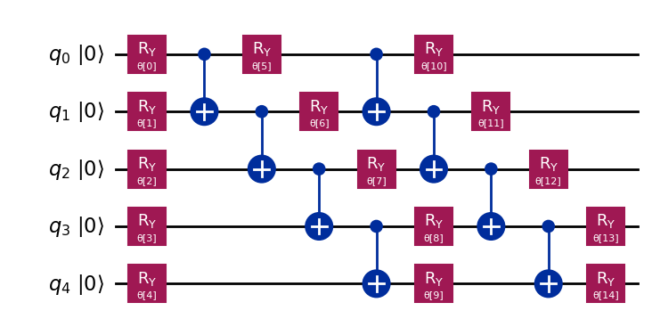
Sometimes we will be interested on generic circuit Ansatze, and we will only want to bound some values to their parametrized gates. \(\texttt{qiskit}\) includes a list of circuits ready to fill only these values; for example n_local:

# This function allows us to feed any entanglement pattern
# with nearest-neighbour, long-range, all-to-all or custom pairing

qc_nn = n_local(5, "ry", "cx", entanglement="linear", reps=2)

qc_lr = n_local(4, "ry", "cx", entanglement=[(0, 1), (1, 3), (0, 3), (2, 3)], reps=2)

In order to feed the parameters, we only need to pass a list of values and assign them:

param_values = rng.uniform(0, 2 * np.pi, qc_lr.num_parameters)
qc_with_values = qc_lr.assign_parameters(param_values)

1.2.2. Plotting circuits

The plotting utility for \(\texttt{qiskit}\) is similar to our draw_layered_circuit function or to the schematic functionality from \(\texttt{quimb}\):

# Drawing the circuit with `mpl` output allows for coloring the gates,
# and `fold=-1`` avoids breaking the circuit
qc.draw(output="mpl", initial_state=True, fold=-1)

qc_nn.draw(output="mpl", initial_state=True, fold=-1)

qc_with_values.draw(initial_state=True, fold=-1)

         ┌────────────┐                ┌────────────┐                         ┌────────────┐              
q_0: |0>─┤ Ry(2.4346) ├──■─────────■───┤ Ry(1.2561) ├───────■──────────────■──┤ Ry(4.4307) ├──────────────
         ├────────────┤┌─┴─┐       │  ┌┴────────────┴┐    ┌─┴─┐            │  ├────────────┤              
q_1: |0>─┤ Ry(1.8116) ├┤ X ├──■────┼──┤ Ry(0.046259) ├────┤ X ├───────■────┼──┤ Ry(4.9055) ├──────────────
         ├────────────┤└───┘  │    │  └──────────────┘┌───┴───┴────┐  │    │  └────────────┘┌────────────┐
q_2: |0>─┤ Ry(4.2882) ├───────┼────┼─────────■────────┤ Ry(4.9444) ├──┼────┼────────■───────┤ Ry(2.8835) ├
        ┌┴────────────┤     ┌─┴─┐┌─┴─┐     ┌─┴─┐      ├────────────┤┌─┴─┐┌─┴─┐    ┌─┴─┐     ├────────────┤
q_3: |0>┤ Ry(0.87809) ├─────┤ X ├┤ X ├─────┤ X ├──────┤ Ry(4.1774) ├┤ X ├┤ X ├────┤ X ├─────┤ Ry(3.5735) ├
        └─────────────┘     └───┘└───┘     └───┘      └────────────┘└───┘└───┘    └───┘     └────────────┘

1.2.3. Recording and loading circuits

A \(\texttt{qiskit}\) circuit can be recorded as a .qasm file. However, because the plotting utility stacks gates according to their order of appearance, information about gate rounds is lost. As a result, there is no need to use the .json recording format in this case, and we therefore do not provide a serialize_from_qiskit_QuantumCircuit function. To address and visualize a circuit coherently on a layer-by-layer basis, one must therefore rely on the functionalities previously introduced for \(\texttt{quimb}\). Nevertheless, when a circuit is produced by the \(\texttt{quimb}\) pipeline, it can indeed be deserialized from a .json file.

generate `qiskit` circuit:
    |
    --> save it:
    |   |
    |   --> .qasm format: `dumps`
    |
    --> load it:
        |
        --> .qasm format: `from_qasm_file`
        |
        --> .json format: `deserialize_to_qiskit_QuantumCircuit`

# Save as `.qasm`
# IMPORTANT: only circuits with bounded parameter values can be dumped in `.qasm`
qasm_code = dumps(qc_with_values)
with open("example_output_qiskit_circuit.qasm", "w") as f:
    f.write(qasm_code)

In \(\texttt{qiskit}\) the .qasm files are loaded as:

qc = QuantumCircuit.from_qasm_file("example_output_quimb_circuit.qasm")

For the sake of completeness, we also introduce a deserialization from .json allowing for loading the circuit until a given depth saved in the key "round" of each "gate":

with open("example_output_quimb_circuit.json") as f:
    dict_loaded_circ = json.load(f)
qc = deserialize_to_qiskit_QuantumCircuit(dict_loaded_circ)

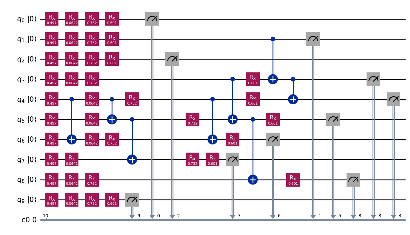
Note that whenever some observable needs to be extracted from the \(\texttt{qiskit}\) circuit instance, a (layer) of measurements must be explicitly called. To activate measures, activate the argument measure=True in deserialize_to_qiskit_QuantumCircuit:

qc = deserialize_to_qiskit_QuantumCircuit(dict_loaded_circ, measure=True)
qc.draw(output="mpl", initial_state=True, fold=-1)

The package \(\texttt{qiskit-quimb}\) is a good option for fast transformation from \(\texttt{qiskit}\) QuantumCircuit into \(\texttt{quimb}\) Circuit classes. Note that the transformation does not include gate round information, so the output \(\texttt{quimb}\) circuit cannot be plotted with draw_layered_circuit:

ent_pattern = [(0, 1), (1, 3), (3, 0), (2, 3), (1, 5), (4, 2), (4, 5), (5, 3)]
qiskit_circ = n_local(6, "h", "cz", entanglement=ent_pattern, reps=2)
quimb_circ = quimb_circuit(qiskit_circ)
quimb_circ.psi.draw(color=[f"I{i}" for i in range(quimb_circ.N)])