7. Robust Phase Estimation

This example introduces the Robust Phase Estimation algorithm; this QPE version requires only a single ancilla/phase qubit. The way the algorithm is implemented is inspired from J.Gunther et al., Phase estimation with partially randomized time evolution arxiv:2503.05647.

In this notebook we explain the idea of the algorithm and apply it to simple models: the Heisenberg model with \(4\) spins, the H\(_2\) molecule in the minimal basis.

We study the Trotter and statistical errors, and check that the RPE algorithm verifies Heisenberg scaling, i.e. the possibility to measure the energy with precision \(\varepsilon\) in time \(\mathcal{O}(1/\varepsilon)\).

import time

import matplotlib.pyplot as plt
import numpy as np
import quimb.tensor as qtn
from pyscf import gto
from tqdm import notebook as tqdm

import qpe_toolbox.estimation as qpe
from qpe_toolbox import EXACT
from qpe_toolbox.hamiltonian import (
    chemistry_hamiltonian,
    do_dmrg,
    heisenberg_hamiltonian,
)

plt.rcParams.update({"font.size": 12})

7.1. Hadamard test

The Robust Phase Estimation algorithm relies on the Hadamard test procedure, which we introduce below. Our presentation takes inspiration from Lin Lin’s lecture notes and the “Hadamard test” Wikipedia page.

The goal of the Hadamard test is to compute \(\bra{\psi} U \ket{\psi}\) where \(U\) is a unitary operator. Since \(U\) is generally not Hermitian, it is not an observable, therefore the real and imaginary part of \(\bra{\psi} U \ket{\psi}\) must be measured separately.

The idea is to build a random variable whose expectation value gives the real (resp. imaginary) part of \(\bra{\psi} U \ket{\psi}\). Consider the following circuit:

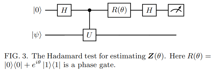
Taken from Günther et al. arXiv:2503.05647.

The Hadamard test uses a single auxiliary qubit initially in state \(\ket{0}\) and a data register with \(n\) qubits initialized in state \(\ket{\psi}\). We start by applying the the Hadamard gate \(H\) to the auxiliary qubit to put it in a superposition state. Then we apply a controlled-\(U\) gate to the data register conditioned on the auxiliary qubit, followed by a a rotation (PHASE) gate \(R(\theta)\) and finally another Hadamard gate on the control qubit.

At the end of the circuit we measure the control qubit and define a random variable \(\textbf{Z}_\theta\): if the result of the measure is \(\ket{0}\), we output \(1\), if the result is \(\ket{1}\) we output \(-1\). The expectation value of \(\textbf{Z}_\theta\) satisfies:

\[ \mathbb{E}\textbf{Z}_\theta = P(0) - P(1) = \mathrm{Re} \left(e^{i\theta} \bra{\psi}U\ket{\psi}\right). \]

We use two special choices of \(\theta\):

\[ \theta = 0 \qquad \implies \qquad \mathbb{E}\textbf{Z}_\theta = \mathrm{Re} \left(\bra{\psi}U\ket{\psi}\right). \]

\[ \theta = -\frac{\pi}{2} \qquad \implies \qquad \mathbb{E}\textbf{Z}_\theta = \mathrm{Im} \left(\bra{\psi}U\ket{\psi}\right). \]

Let \(\textbf{X}\) and \(\textbf{Y}\) be the random variables corresponding to \(\theta=0, -\pi/2\) respectively. Define \(\textbf{Z} = \textbf{X} + i \textbf{Y}.\) Then we get

\[ \mathbb{E}\textbf{Z} = \bra{\psi}U\ket{\psi} \]

Let us first illustrate a simple instance of the Hadamard test with \(U = |0\rangle \langle 0| + e^{i\alpha} |1\rangle \langle 1|\) and \(|\psi\rangle = |1\rangle\).

alpha = np.pi / 6
print(f"cos(alpha) = {np.cos(alpha):.4g} and sin(alpha) = {np.sin(alpha):.4g}")

# Hadamard test with theta=0
circ = qtn.Circuit(2)
circ.apply_gate("X", 1)
circ.apply_gate("H", 0)
circ.apply_gate("CPHASE", alpha, 0, 1)
circ.apply_gate("H", 0)

probs = circ.compute_marginal(where=[0])
print(f"Re(<psi|U|psi>) = {probs[0] - probs[1]:.4g}")

# Hadamard test with theta=-pi/2
circ = qtn.Circuit(2)
circ.apply_gate("X", 1)
circ.apply_gate("H", 0)
circ.apply_gate("CPHASE", alpha, 0, 1)
circ.apply_gate("PHASE", -np.pi / 2, 0)
circ.apply_gate("H", 0)

probs = circ.compute_marginal(where=[0])
print(f"Im(<psi|U|psi>) = {probs[0] - probs[1]:.4g}")

cos(alpha) = 0.866 and sin(alpha) = 0.5

Re(<psi|U|psi>) = 0.866
Im(<psi|U|psi>) = 0.5

Now take the Heisenberg Hamiltonian with \(4\) spins

n_qubits = 4
H = heisenberg_hamiltonian(n_qubits)
E0, psi0 = do_dmrg(H)

We run the Hadamard test on the time evolution operator \(U = e^{-iHt}\) with the physical register in state \(\ket{\psi} = \ket{\psi_0}\). Then

\[ \mathbb{E}\textbf{Z} = e^{-i E_0 t}. \]

The function run_hadamard_test runs the Hadamard test and returns \(\mathrm{Re}~e^{i\theta} \bra{\psi}U\ket{\psi}\).

Below we estimate \(E_0\) by running the Hadamard test for a time evolution during a random time \(t\).

We first consider exact time evolution.

rng = np.random.default_rng(seed=42)
t = rng.random()
data_reg = list(range(1, n_qubits + 1))
U = H.get_U_exact(t, data_reg, controls=(0,))

n_shots = EXACT  # exact computation (no sampling)

X = qpe.run_hadamard_test(psi0, U, 0, n_shots)
Y = qpe.run_hadamard_test(psi0, U, -np.pi / 2, n_shots)
Z = X + 1j * Y

print(f"error = {abs(np.angle(Z) / t + E0):.2g}")

error = 4.4e-08

The previous relation defines a function \(g: t \to \mathbb{E}\textbf{Z}(t) \).

At this stage let us emphasize two points:

• In general:

\[ \mathbb{E}\textbf{Z}(t) = \sum_k c_k e^{i E_k t}, \qquad \text{where} \qquad H\ket{\psi_k} = E_k \ket{\psi_k},~c_k = |\langle \psi | \psi_k \rangle|^2. \]

In the following, we consider the simplest case \(c_0=1\) (\(\psi\) is the ground state).

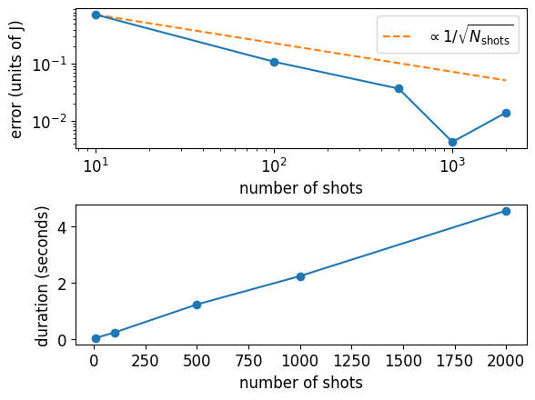
• With a QPU emulator like \(\texttt{quimb}\), the probabilities \(P(0)\), \(P(1)\) can be computed exactly. On a real quantum device, these probabilities are estimated from repeated measurements (shots). With a finite number of shots \(N_{\rm shots}\), we can estimate \(g(t)\) by taking the statistical mean over \(N_{\rm shots}\) samples:

\[ \bar{\bf Z}(t) = \frac{1}{N_{\rm shots}} \sum_{n=1}^{N_{\rm shots}} {\bf Z}^{(n)} (t). \]

If \(N_{\rm shots}\) shots are used, the statistical error scales as

\[\mathcal{O}\left(\frac{1}{\sqrt{N_{\rm shots}}}\right).\]

shots_list = np.array([10, 100, 500, 1000, 2000])
errors = []
durations = []

for n_shots in tqdm.tqdm(shots_list):
    st = time.time()
    X = qpe.run_hadamard_test(psi0, U, 0, n_shots=n_shots)
    Y = qpe.run_hadamard_test(psi0, U, -np.pi / 2, n_shots=n_shots)
    et = time.time() - st

    Z = X + 1j * Y
    error = abs(np.angle(Z) / t + E0)

    errors.append(error)
    durations.append(et)

The statistical error decreases as \(1/\sqrt{N_{\rm shots}}\) while the computation time increases linearly with \(N_{\rm shots}\)

fig, (ax_e, ax_t) = plt.subplots(nrows=2)
fig.subplots_adjust(hspace=0.4)
ax_e.loglog(shots_list, errors, "-o")
ax_e.loglog(
    shots_list,
    errors[0] * np.sqrt(10 / shots_list),
    "--",
    label="$\\propto 1/\\sqrt{N_{\\rm shots}}$",
    zorder=0,
)
ax_t.plot(shots_list, durations, "-o")
ax_e.legend()
ax_e.set_xlabel("number of shots")
ax_t.set_xlabel("number of shots")
ax_e.set_ylabel("error (units of J)")
ax_t.set_ylabel("duration (seconds)");

7.2. Robust phase estimation algorithm

7.2.1. Introduction

Quote from Günther et al. arxiv:2503.05647:

“If we think of g(t) as a time signal, then the phase estimation routine will constitute a signal processing transformation to compute the lowest frequency of \(g(t)\) (corresponding to the energy \(E_0\)), provided that we have some guarantee on the overlap of \(\ket{\psi}\) with the ground state; we assume a lower bound \(c_0 \geq \eta\). With appropriate signal processing methods, one can find the value of \(E_0\) with accuracy \(\varepsilon\) using \(M\) circuits with time evolution for times \(t_1, . . . , t_M\). This can be done such that the maximal time evolution \(t_{\rm max} = \mathrm{max}\{t_1, . . . , t_M\}\) and the total time over all circuit runs \(t_{\rm tot} = t_1 + t_2 + · · · + t_M\) both scale as \(\varepsilon^{-1}\). This Heisenberg scaling is known to be optimal.”

7.2.2. Algorithm

To get precision \(\varepsilon\), the idea of the robust phase estimation algorithm is to consider \(M\) different circuits where \(M = \lceil \log_2 \varepsilon^{-1} \rceil\) and estimate

\[ g(2^m) = \mathbb{E}[Z(2^{m})] = \exp(-i 2^{m} E_0) \]

for \(m=0,1,..,M-1\). Each iteration gives a supplementary bit of precision on \(E_0\).

Algorithm 1 (p.24)

1. The algorithm is initialized with \(\theta_{-1}=0\) so that \(\theta_0 = \phi_0\).

2. For each \(m\):

   • Take \(N_{\rm shots}\) samples to compute the average:

   \[ \bar{\bf Z}(2^{m}) = \frac{1}{N_{\rm shots}} \sum_{n=1}^{N_{\rm shots}} {\bf Z}^{(n)} (2^m) \]

   • From the outcome we compute \(\phi_m = - \arg(\bar{Z}(2^m))\) using numpy.angle

   • By definition \(\phi_m \in ]-\pi, \pi]:~\phi_m~\) is an approximation of \(2^mE_0\) modulo \(2\pi\)

   • Given a previous guess \(\theta_{m-1}\) for the ground state energy \(E_0\), the new energy estimate \(\theta_m\) is given by

   \[ \theta_m = 2^{-m} (2\pi k + \phi_m), \]

   where \(k\) is an integer between \(0\) and \(2^m - 1\) which minimizes the distance

   \[ d(\theta_m, \theta_{m-1}) = \min_{q\in\mathbb{Z}} | \theta_m - \theta_{m-1} + 2q\pi|, \]

   under the condition \(-\pi < \theta \leq \pi\).

The algorithm ensures that at each step, \(\theta_m\) is the best \(m\)-bit approximation of \(E_0\). The following lemma guarantees convergence:

Lemma B.1. (p.25): if \(d(\phi_k,2^{k}E)<\frac{\pi}3\) for \(k=0,1,...,m\) then \(\theta_m\) is such that \(d(\theta_m,E) \leq 2^{-m}\frac{\pi}3\)

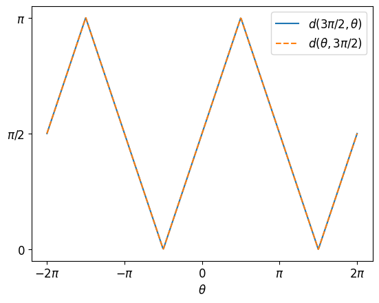
7.2.2.1. Illustration of the distance \(d(\theta,\phi)\)

To build an intuition, let us plot the distance \(d(\theta, \phi)\) as a function of \(\theta\) for a given \(\phi\) (\( 3\pi/2\) in the example) and vice-versa (the distance is symmetric by definition).

thetas = np.linspace(-2 * np.pi, 2 * np.pi, 600)
plt.xticks(
    [i * np.pi for i in range(-2, 3)],
    [r"$-2\pi$", r"$-\pi$", "$0$", r"$\pi$", r"$2\pi$"],
)
plt.yticks([0, np.pi / 2, np.pi], ["0", "$\\pi/2$", "$\\pi$"])

plt.xlabel(r"$\theta$")

plt.plot(
    thetas,
    [qpe.rpe_distance(t, 3 * np.pi / 2) for t in thetas],
    label=r"$d(3\pi/2, \theta)$",
)
plt.plot(
    thetas,
    [qpe.rpe_distance(3 * np.pi / 2, t) for t in thetas],
    "--",
    label=r"$d(\theta, 3\pi/2)$",
)
plt.legend();

Let us now illustrate the first two steps of the algorithm for concreteness. We start with \(N_{\rm shots}=2\) and \(\epsilon = 0.2\). We also consider exact time evolution.

sign_E0 = np.sign(E0)

epsilon = 0.02
M = int(np.ceil(np.log2(1 / epsilon)))

n_shots = 2

# m = 0
phi_0 = qpe.rpe_get_hadamard_output(H, psi0, 0, EXACT, n_shots)
theta_0 = phi_0

m = 1
phi_1 = qpe.rpe_get_hadamard_output(H, psi0, m, EXACT, n_shots)
S_1 = [(phi_1 + sign_E0 * 2 * np.pi * k) / 2**m for k in range(2**m)]

Let’s visualize how the different elements of \(S_1\) compare to \(\theta_0\)

plt.hlines(1, -np.pi, np.pi, "k")
plt.plot([-np.pi, np.pi], [1, 1], "|", markersize=10, color="k")
plt.plot(theta_0, 1, "*", markersize=20, color="r", label=r"$\theta_0$")
y = np.ones(np.shape(S_1))
plt.plot(S_1, y, "o", markersize=15, label=r"$S_1$")

plt.text(-1.1 * np.pi, 0.99, r"$-\pi$", fontsize=16)
plt.text(np.pi, 0.99, r"$\pi$", fontsize=16)
plt.text(1.05 * theta_0, 0.99, r"$\theta_0$", fontsize=16, color="r")

plt.axis("off")
plt.legend();

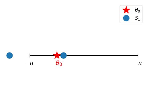
We compute \(\theta_1\) as the element from \(S_1\) closest to \(\theta_0\) and check that the error decreases between the first and second iteration:

theta_1, d_min = qpe.rpe_update_theta(S_1, theta_0)
print(f"Exact energy E = {E0:.4f}")
print(f"theta_0 = {theta_0:.4f}")
print(f"theta_1 = {theta_1:.4f}")

Exact energy E = -1.6160
theta_0 = -2.3562
theta_1 = -1.1781

7.2.3. Run RPE. Statistical precision

We will now run the algorithm and see the influence of statistical noise. The robust_phase_estimation function returns the full list of \(\theta_m\), \(m=0,...,M-1\).

We start with \(N_{\rm shots}=1\).

epsilon = 0.02
M = int(np.ceil(np.log2(1 / epsilon)))
print(f"Target precision epsilon={epsilon}: requires M={M} iterations\n")

n_shots = 1

theta_list = qpe.robust_phase_estimation(
    H, psi0, epsilon, sign_E0, EXACT, n_shots, verbosity=1
)

Target precision epsilon=0.02: requires M=6 iterations

m 	 phi_m  	 theta_m 	 time (s)
0 	 -0.7854 	 -0.7854 	 0.0   
1 	 -2.3562 	 -1.1781 	 0.0   
2 	 -0.7854 	 -1.7671 	 0.1   
3 	 0.7854 	 -1.4726 	 0.1   
4 	 -0.7854 	 -1.6199 	 0.1   
5 	 -2.3562 	 -1.6444 	 0.1   
6 	 -2.3562 	 -1.6076 	 0.1   

plt.semilogy(
    [qpe.rpe_distance(theta, E0) for theta in theta_list[1:]],
    "-o",
    label=f"$N_{{\\rm shots}}={n_shots}$",
)
plt.semilogy([np.pi / 3 / 2**i for i in range(M + 1)], "k--", label="$2^{-m}~\\pi/3$")
plt.legend()
plt.xlabel("iteration $m$")
plt.ylabel("$d(\\theta_m, E)$");

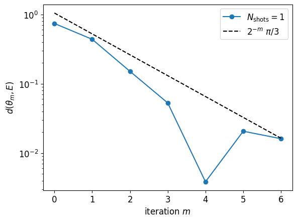
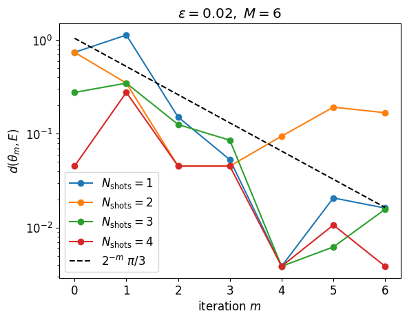
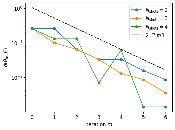
We see that for such small systems, with exact time evolution, a single shot gives an estimate that converges. We now increase the number of shots to improve the precision

n_shot_list = [1, 2, 3, 4]

for n_shots in n_shot_list:
    theta_list = qpe.robust_phase_estimation(H, psi0, epsilon, sign_E0, EXACT, n_shots)
    plt.semilogy(
        [qpe.rpe_distance(theta, E0) for theta in theta_list[1:]],
        "-o",
        label=f"$N_{{\\rm shots}}={n_shots}$",
    )

plt.semilogy([np.pi / 3 / 2**i for i in range(M + 1)], "k--", label="$2^{-m}~\\pi/3$")
plt.legend()
plt.xlabel("iteration $m$")
plt.ylabel("$d(\\theta_m, E)$")
plt.title(rf"$\epsilon={epsilon},\; M={M}$");

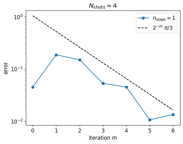
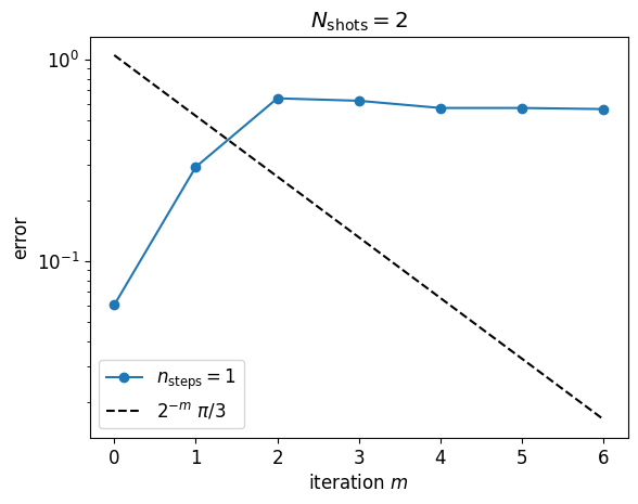
7.2.4. Trotter approximation of the time evolution operator

We now apply the same algorithm but replace the exact time evolution operator by a second order Trotter approximation.

The n_steps argument in the robust_phase_estimation function sets the number of Trotter steps for \(m=0\). The number of steps is multiplied by \(2\) at each iteration to keep the Trotter timestep constant.

The computation will now take longer since the number of gates for the time evolution now grows like \(2^m\).

%%time
print(f"epsilon={epsilon}, M={M}")

n_steps = 1
n_shots = 4
thetas_ttr_list = []

thetas_ttr = qpe.robust_phase_estimation(
    H, psi0, epsilon, sign_E0, n_steps, n_shots, verbosity=1
)

thetas_ttr_list.append(thetas_ttr)

epsilon=0.02, M=6
m 	 phi_m  	 theta_m 	 time (s)

0 	 -1.5708 	 -1.5708 	 0.5   

1 	 -3.1416 	 -1.5708 	 1.3   

2 	 -0.4636 	 -1.6867 	 3.1   

3 	 -0.7854 	 -1.669 	 6.6   

4 	 -0.7854 	 -1.6199 	 13.5  

5 	 -0.7854 	 -1.5953 	 27.3  

6 	 -2.0344 	 -1.6026 	 54.7  
CPU times: user 55 s, sys: 520 ms, total: 55.5 s
Wall time: 54.7 s

plt.semilogy(
    [qpe.rpe_distance(theta, E0) for theta in thetas_ttr_list[0][1:]],
    "-o",
    label=f"$n_{{\\rm steps}}={n_steps}$",
)
plt.semilogy([np.pi / 3 / 2**i for i in range(M + 1)], "k--", label="$2^{-m}~\\pi/3$")
plt.legend()
plt.title(r"$N_{\rm shots}=4$")
plt.xlabel("iteration $m$")
plt.ylabel("error");

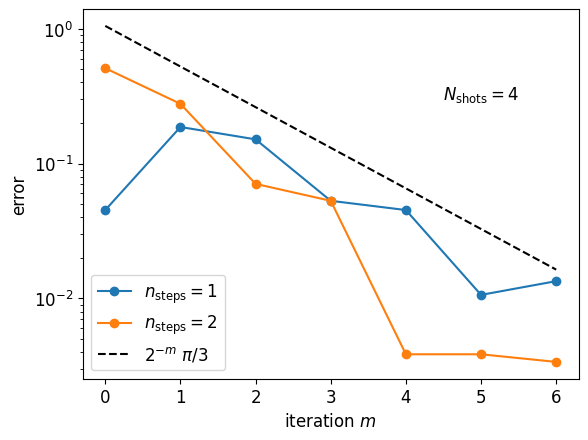
Let us increase the number of Trotter steps. This will take a few minutes

%%time

n_steps = 2
thetas_ttr = qpe.robust_phase_estimation(
    H, psi0, epsilon, sign_E0, n_steps, n_shots, verbosity=1
)
thetas_ttr_list.append(thetas_ttr)

m 	 phi_m  	 theta_m 	 time (s)
0 	 -1.1071 	 -1.1071 	 0.9   
1 	 -3.1416 	 -1.5708 	 2.7   

2 	 -0.7854 	 -1.7671 	 6.1   

3 	 -0.4636 	 -1.6288 	 13.1  

4 	 -0.7854 	 -1.6199 	 26.8  

5 	 -1.5708 	 -1.6199 	 53.9  

6 	 -2.6779 	 -1.6126 	 108.0 
CPU times: user 1min 48s, sys: 796 ms, total: 1min 49s
Wall time: 1min 47s

for i, n_steps in enumerate([1, 2]):
    plt.semilogy(
        [qpe.rpe_distance(theta, E0) for theta in thetas_ttr_list[i][1:]],
        "-o",
        label=f"$n_{{\\rm steps}}={n_steps}$",
    )

plt.semilogy([np.pi / 3 / 2**i for i in range(M + 1)], "k--", label="$2^{-m}~\\pi/3$")
plt.legend()
plt.text(4.5, 0.3, "$N_{\\rm shots}=4$")
plt.xlabel("iteration $m$")
plt.ylabel("error");

7.3. Heisenberg scaling

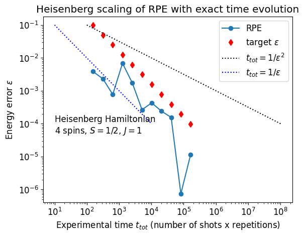
The experimental time is proportional to \(N_{\rm shots} \sum_{m=0}^M 2^m\), i.e. it scales like \(2^M\). The RPE algorithm reaches a precision \(\varepsilon\) in \(M = \lceil \log_2 \varepsilon^{-1} \rceil\) iterations. Hence it achieves Heisenberg scaling: reaching a precision \(\varepsilon\) in time \(\mathcal{O}(2^M) = \mathcal{O}(1/\varepsilon)\).

Let us illustrate that below: we run the RPE algorithm for various \(\varepsilon\) and plot experimental time versus energy error. (We take exact time evolution for simplicity: in this case we consider that the experimental time is exactly \(N_{\rm shots} \sum_{m=0}^M 2^m\).)

epsilon_list = [0.1 / 2**m for m in range(11)]
n_shots = 5

cost_list = []
res_list = []
for epsilon in epsilon_list:
    M = int(np.ceil(np.log2(1 / epsilon)))
    cost_list.append(sum([n_shots * 2**m for m in range(M + 1)]))
    theta_list = qpe.robust_phase_estimation(H, psi0, epsilon, sign_E0, EXACT, n_shots)
    res_list.append(theta_list[-1])

plt.loglog(cost_list, [abs(en - E0) for en in res_list], "-o", label="RPE")
plt.loglog(cost_list, epsilon_list, "rd", label=r"target $\epsilon$")
plt.loglog(
    [1 / eps**2 for eps in epsilon_list],
    epsilon_list,
    "k:",
    label=r"$t_{tot}=1/\epsilon^2$",
)
plt.loglog(
    [1 / eps for eps in epsilon_list], epsilon_list, "b:", label=r"$t_{tot}=1/\epsilon$"
)

plt.xlabel("Experimental time $t_{tot}$ (number of shots x repetitions)")
plt.ylabel(r"Energy error $\epsilon$")
plt.title("Heisenberg scaling of RPE with exact time evolution")
plt.text(10, 5e-5, "Heisenberg Hamiltonian \n4 spins, $S=1/2$, $J=1$")
plt.legend();

7.4. Quantum chemistry example: diatomic Hydrogen

Let us now consider a molecule: we take \(H_2\) in the minimal atomic orbital basis STO-3G. The Hamiltonian in qubit form is obtained via a Jordan-Wigner transformation. Contrary to the previous spin Hamiltonian, the molecular Hamiltonian is non-local: it couples qubits at long distance.

mol = gto.M(
    atom=[("H", (0.0, 0.0, 0.0)), ("H", (0.0, 0.0, 0.735))],
    basis="STO-3G",
)

H_H2 = chemistry_hamiltonian(
    mol, hf_mode="rhf", encoding="original", do_fci=True, do_ccsd=False
)
E0_H2, psi0_H2 = do_dmrg(H_H2)
print(f"E_DMRG : {E0_H2 + H_H2.e_const:.10f}")

converged SCF energy = -1.116998996754

nOrb   : 2
nElec  : 2
E_HF   : -1.1169989968

E_CI   : -1.1373060358

E_DMRG : -1.1373060358

7.4.1. Exact time evolution

The system is small enough for exact exponentiation of the Hamiltonian matrix, and exact time evolution

epsilon = 0.02
M = int(np.ceil(np.log2(1 / epsilon)))
sign_E0 = np.sign(E0_H2)
n_shot_list = [2, 3, 4]

for n_shots in n_shot_list:
    theta_list = qpe.robust_phase_estimation(
        H_H2, psi0_H2, epsilon, sign_E0, EXACT, n_shots
    )
    plt.semilogy(
        [qpe.rpe_distance(theta, E0_H2) for theta in theta_list[1:]],
        "-o",
        label=f"$N_{{\\rm shots}}={n_shots}$",
    )

plt.semilogy([np.pi / 3 / 2**i for i in range(M + 1)], "k--", label="$2^{-m}~\\pi/3$")
plt.legend()
plt.xlabel("iteration $m$")
plt.ylabel("$d(\\theta_m, E)$");

7.4.2. Trotter

The Trotter decomposition of the molecular Hamiltonian is longer, and simulations become harder. The following run will take a minute…

%%time
n_shots = 2
n_steps = 1

thetas_ttr = qpe.robust_phase_estimation(
    H_H2, psi0_H2, epsilon, sign_E0, n_steps, n_shots, verbosity=1
)

m 	 phi_m  	 theta_m 	 time (s)
0 	 -0.7854 	 -0.7854 	 0.7   

1 	 -1.5708 	 -0.7854 	 2.2   

2 	 1.5708 	 -1.1781 	 5.1   

3 	 -1.5708 	 -0.9817 	 11.0  

4 	 2.3562 	 -1.0308 	 22.2  

5 	 -1.5708 	 -1.0308 	 44.8  

6 	 1.5708 	 -1.0554 	 89.5  
CPU times: user 1min 30s, sys: 625 ms, total: 1min 30s
Wall time: 1min 29s

… and fails to get the desired precision

plt.semilogy(
    [qpe.rpe_distance(theta, E0_H2) for theta in thetas_ttr_list[i][1:]],
    "-o",
    label=f"$n_{{\\rm steps}}={n_steps}$",
)

plt.semilogy([np.pi / 3 / 2**i for i in range(M + 1)], "k--", label="$2^{-m}~\\pi/3$")
plt.legend()
plt.title(f"$N_{{\\rm shots}}={n_shots}$")
plt.xlabel("iteration $m$")
plt.ylabel("error");

If you want to reach the expected precision, what would you try to increase first? \(N_{\rm shots}\) or \(n_{\rm steps}\)?

7.4.3. Chemical accuracy?

The standard for chemical accuracy is \(\varepsilon = 10^{-3}\) Ha. Hartrees are the default unit in pyscf. We can compute directly the number of iterations required for chemical accuracy:

epsilon = 0.001
M = int(np.ceil(np.log2(1 / epsilon)))
print(f"Chemical accuracy eps={epsilon} requires M={M} iterations")

Chemical accuracy eps=0.001 requires M=10 iterations

Reaching chemical accuracy requires at least ten iterations, and a sufficient number of shots and Trotter steps. If you want to go further, you can first make an estimation of the runtime for \(M=10\) and a given number of shots and Trotter steps, then with some patience try to run the simulation.