5. QPE with Trotterization

In this example we perform Quantum Phase Estimation with a second-order Trotter decomposition of the time evolution operator \(U(t) = \exp(-i H t)\).

Previously in the Textbook QPE example, we introduced and ran QPE with an exact matrix representation of \(U\); this is only possible for small systems amenable to exact diagonalization. In general, we use a Trotter approximation to exponentiate the Hamiltonian; see the tutorial on Trotter-Suzuki decomposition for an introduction to Trotter approximants to exponentials of matrices.

We study the precision obtained on the energy as a function of the number of phase qubits in the QPE circuits and the number of Trotter steps in the time evolution. We also perform some simple resource analysis: we quantify the number of entangling gates and the time required to simulate the circuits with \(\texttt{quimb}\).

import matplotlib.pyplot as plt
import numpy as np
from tqdm import notebook as tqdm

import qpe_toolbox.estimation as qpe
from qpe_toolbox import EXACT
from qpe_toolbox.circuit import count_gates_by_qb, make_circ, make_circMPS
from qpe_toolbox.hamiltonian import do_dmrg, heisenberg_hamiltonian

plt.rcParams.update({"font.size": 12})

mystyles = [
    {"linestyle": "--", "linewidth": 1, "color": "black"},
    {"linestyle": ":", "marker": "o", "markersize": 10, "color": "tab:blue"},
    {"linestyle": ":", "marker": "s", "markersize": 8, "color": "tab:orange"},
    {"linestyle": ":", "marker": "v", "markersize": 8, "color": "tab:green"},
    {"linestyle": ":", "marker": "*", "markersize": 10, "color": "tab:red"},
    {"linestyle": ":", "marker": "^", "markersize": 8, "color": "tab:brown"},
]

5.1. Introduction

• We consider the 1D nearest-neighbour Heisenberg Hamiltonian with open boundary conditions and take the DMRG ground state as the “exact” reference state.

n_qubits = 4
h_spin = heisenberg_hamiltonian(n_qubits)
exact_energy, psi0_mps = do_dmrg(h_spin)

• Then we set the different parameters to compute the energy with QPE. The QPE circuit output is a phase \(2 \pi \theta\). We need to set an appropriate global phase and total evolution time to make sure we recover the correct energy value from the output \(\theta\) (see the example on Textbook QPE ).

• Note that the number of Trotter steps (which we denote by n_trotter_steps or n_steps) gives the number of Trotter steps to decompose the time interval \(t\) (evolution_time) i.e. it sets the number of substeps for the first controlled time evolution. Along the circuit, we apply time evolution over an exponentially growing time \(2^k t\) conditioned on the \(k\)-th circuit; the number of Trotter steps grows accordingly as \(2^k\) so as to keep the Trotter timestep constant.

E_target = exact_energy + 0.2
size_interval = 2
Emax = E_target + size_interval / 2
evolution_time = 2 * np.pi / size_interval
global_phase = Emax * evolution_time

print(f"exact theta = {(E_target + size_interval / 2 - exact_energy) / size_interval}")

n_phase_bits0 = 2
n_trotter_steps0 = 1
print(
    f"Precision on theta = {1 / 2**n_phase_bits0}, precision on energy = {1 / 2**n_phase_bits0 * size_interval}\n"
)

circuit0 = make_circ(n_phase_bits0, psi0_mps)
trotter_order0 = 1

exact theta = 0.6
Precision on theta = 0.25, precision on energy = 0.5

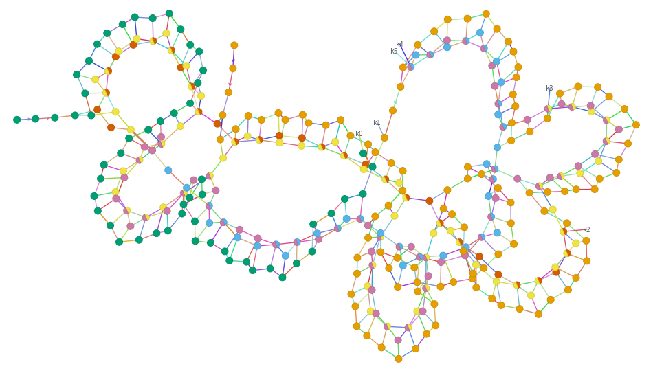
• \(\texttt{quimb}\) represents the QPE circuit as a tensor network:

dt = evolution_time / n_trotter_steps0
_, circ = qpe.qpe_first_stage(
    h_spin, circuit0, evolution_time, dt, global_phase, trotter_order=trotter_order0
)

phase_reg = list(range(n_phase_bits0))
circ.apply_gates(qpe.iqft_swapped(phase_reg))

circ.psi.draw(
    figsize=(12, 12),
    show_tags=False,
    color={f"I{i}" for i in range(n_qubits + n_phase_bits0)},
    edge_scale=1,
    layout="kamada_kawai",
    edge_color=True,
    legend=False,
)

• We compute the energy and make sure the precision is within the theoretical error bound:

traces, energy = qpe.qpe_energy(
    h_spin,
    circuit0,
    n_trotter_steps0,
    E_target,
    size_interval,
    trotter_order=trotter_order0,
    verbosity=1,
)

print(f"\nBest guess = {energy:.4f} with proba {traces['prob']:.4f}")
print(f"exact energy = {exact_energy:.4f}")

# check error is below QPE upper bound
print(
    f"error = {abs(exact_energy - energy):.4f} < error bound = {size_interval / 2**n_phase_bits0:.4f}"
)

10 |2> 0.5  0.6581

01 |1> 0.25 0.1777

00 |0> 0.0  0.0936

11 |3> 0.75 0.0706

Best guess = -1.4160 with proba 0.6581
exact energy = -1.6160
error = 0.2000 < error bound = 0.5000

5.2. Precision: influence of the number of phase qubits and number of Trotter steps

We run and measure the energy for several QPE circuits varying the number of phase qubits and Trotter steps. We also record the gate count and simulation time, and compare two modes of circuit simulation available with \(\texttt{quimb}\): the Circuit mode and the CircuitMPS mode. For the Circuit mode we choose a greedy hyperoptimizer, see our notebook on Hyperoptimization.

Let us first run the circuits (this may take a couple of minutes):

res = {"durations_tn": [], "durations_mps": [], "energies": [], "entangling_gates": []}
trotter_order = 2
nphase_list = np.array([1, 2, 3, 4, 5])
ns_list = [1, 2, 3, 4, EXACT]
max_tn_nphase = 5
max_tn_nsteps = 3

for n_trotter_steps in tqdm.tqdm(ns_list):
    duration_tn = []
    duration_mps = []
    energies = []
    gates_count = []
    for n_phase_bits in tqdm.tqdm(nphase_list, leave=False):
        initial_circMPS = make_circMPS(n_phase_bits, psi0_mps)

        if (n_trotter_steps is not EXACT) and (
            n_phase_bits < max_tn_nphase or n_trotter_steps < max_tn_nsteps
        ):
            # using generic tensor network contraction to simulate a quantum circuit
            # is usually very expensive. Only try for small number of qubits.
            initial_circ = make_circ(n_phase_bits, psi0_mps)
            traces, energy = qpe.qpe_energy(
                h_spin,
                initial_circ,
                n_trotter_steps,
                E_target,
                size_interval,
                trotter_order=trotter_order,
                optimize="greedy",
            )
            duration_tn.append(traces["ctimes"][-1])

        # contracting circuit in MPS mode is much more efficient
        # deeper, wider circuits can be classicaly simulated
        traces, energy = qpe.qpe_energy(
            h_spin,
            initial_circMPS,
            n_trotter_steps,
            E_target,
            size_interval,
            trotter_order=trotter_order,
        )
        energies.append(energy)
        count = count_gates_by_qb(traces["gates_count"])
        gates_count.append(count["2qb"] + count["3+qb"])
        duration_mps.append(traces["ctimes"][-1])
        assert abs(energy - energies[-1]) < 1e-6

    res["durations_tn"].append(duration_tn)
    res["energies"].append(np.array(energies))
    res["durations_mps"].append(duration_mps)
    res["entangling_gates"].append(gates_count)

5.2.1. Error versus number of phase qubits

Let us see how the precision improves when adding more qubits in the phase register, for different number of Trotter steps:

fig, ax = plt.subplots()
ax.plot(
    nphase_list,
    size_interval / 2**nphase_list,
    label="$\\Delta/2^{n_{\\rm phase~bits}}$",
    **mystyles[0],
)
ax.plot(
    nphase_list,
    np.abs(res["energies"][-1] - exact_energy),
    label="exact time evolution",
    **mystyles[1],
)
for i, n_trotter_steps in enumerate(ns_list[:-1]):
    ax.plot(
        nphase_list,
        np.abs(res["energies"][i] - exact_energy),
        label=f"{n_trotter_steps} Trotter steps",
        **mystyles[i + 2],
    )
ax.legend(loc="lower right", bbox_to_anchor=(1.5, 0.4))
ax.set_ylim(0, 0.25)
ax.set_xticks(range(1, 6))
ax.set_xlabel("number of phase qubits")
ax.set_ylabel("energy error");

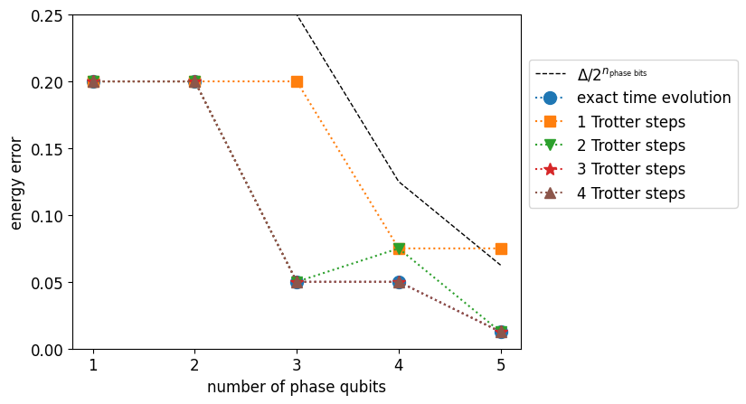
\(\Delta=\) size_interval is the size of the search window \([E_{\rm target} - \Delta/2, E_{\rm target} + \Delta/2]\) where we expect to find \(E_0\), see the first example on Textbook QPE. The black dashed curve \(\Delta/2^{n_{\rm phase~bits}}\) is the upper bound of QPE error.

For n_trotter_steps >= 3, the Trotter error becomes negligible and the curves overlap with exact time evolution.

5.2.2. Error versus number of Trotter steps

We now plot the error as a function of the number of Trotter steps \(n_{\rm steps}\) for a given number of phase qubits:

energies = np.array([res["energies"][i][-1] for i in range(len(ns_list) - 1)])

fig, ax = plt.subplots()
xfit = np.linspace(1, 5, 41)
ax.plot(
    xfit,
    abs(energies[0] - exact_energy) * (ns_list[1] / xfit) ** 2,
    linestyle="--",
    color="r",
    label="$\\mathcal{O}(t^3/n_{\\rm steps}^2)$",
)
ax.axhline(
    y=size_interval / 2 ** nphase_list[-1],
    linestyle=":",
    color="k",
    label="$\\Delta/2^{n_{\\rm phase~bits}}$",
)
ax.plot(
    ns_list[:-1],
    np.abs(energies - exact_energy),
    label=f"{nphase_list[-1]} phase qubits",
    **mystyles[1],
)
ax.legend(loc="upper right", framealpha=1)
ax.set_xticks(range(1, 5))
ax.set_xlim(0.8, 4.2)
ax.set_ylim(0, 0.14)
ax.set_xlabel("number of Trotter steps")
ax.set_ylabel("energy error");

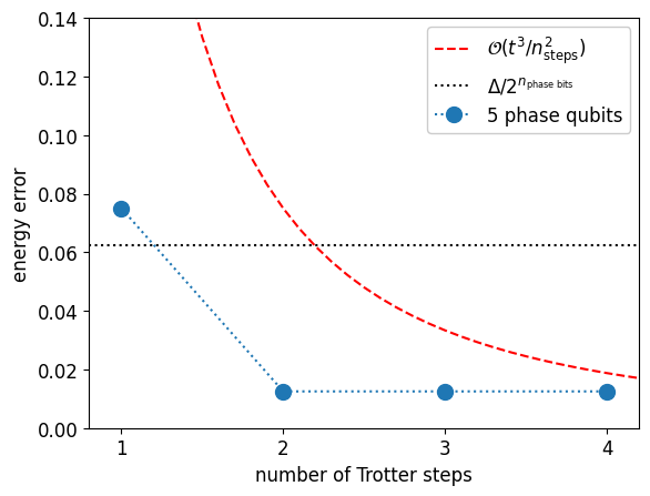
The red dashed line shows the second order Trotter error bound \(t^3 / n_{steps}^2\). The black dashed line shows the theoretical QPE error bound \(\Delta / 2^{n_{\rm phase qubits}}\). Here \(2\) Trotter steps are sufficient to reach the QPE precision for this number of phase qubits.

5.2.3. Gate count and computation time

Let us now visualize the gate count. We only count entangling gates, i.e. not one-qubit gates. The Trotterized time-evolution operator is implemented with CNOT gates and single qubit gates (rotations). In QPE, the time-evolution is controlled on the phase register. Hence, the CNOT become multi-controlled CCNOT gates and the rotation gates become controlled-rotations. Since the number of Trotter steps along the controlled time evolution sequence grows exponentially with the number of phase qubits, so does the number of entangling gates.

fig, (ax_n, ax_t) = plt.subplots(1, 2, figsize=(12, 4))

for i, n_trotter_steps in enumerate(ns_list[:-1]):
    ax_n.plot(
        nphase_list,
        res["entangling_gates"][i],
        label=f"{n_trotter_steps} steps",
        **mystyles[i + 2],
    )
    ax_t.plot(
        nphase_list,
        res["durations_mps"][i],
        label=f"{n_trotter_steps} steps MPS",
        **mystyles[i + 2],
    )

# Plot TN timings on top
for i, n_trotter_steps in enumerate(ns_list[:-1]):
    ax_t.plot(
        nphase_list[nphase_list < max_tn_nphase]
        if n_trotter_steps >= max_tn_nsteps
        else nphase_list,
        res["durations_tn"][i],
        label=f"{n_trotter_steps} steps TN",
        marker="P",
        markersize=8,
        linestyle="--",
        markeredgecolor="k",
        color=mystyles[i + 2]["color"],
    )

ax_n.legend(fontsize=12)
ax_t.legend()
ax_n.set_xlabel("number of phase qubits")
ax_n.set_ylabel("number of entangling gates")
ax_t.set_xlabel("number of phase qubits")
ax_t.set_ylabel("computation time (seconds)");

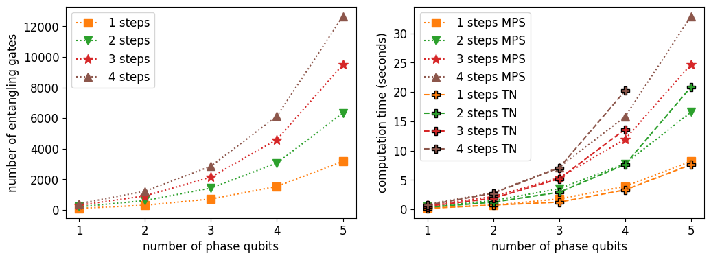
• The CircuitMPS mode is much more efficient than the Circuit mode (actual timing depends on the contraction order found by the optimizer, see our notebook on Hyperoptimization). The computation time is directly correlated with the number of entangling gates, which grows exponentially with the number of phase qubits.

• We quickly reach computation times of tens of seconds due to the exponentially growing circuit depth. Recall that for such small systems, the Hamiltonian can be exactly diagonalized in a fraction of a second on any laptop. We know that for QPE to gain an advantage compared to exact diagonalization or DMRG, larger systems, with more than 30 qubits and strong correlations, must be considered.

• Note that a comparison between \(\texttt{quimb}\)’s CircuitMPS and \(\texttt{qiskit}\) MPS can be found in the Performance MPS example. A detailed example on the way \(\texttt{quimb}\) performs tensor network contraction and in particular hyperoptimization can be found in the Hyperoptimization notebook.

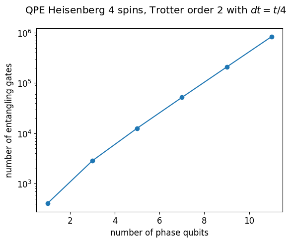
5.3. Resource analysis

For larger number of phase qubits, computation becomes costly: in the following we do not run the simulation but just get the list of gate instructions

E_const, Emax, evolution_time_resource, global_phase_resource = qpe.set_search_window(
    h_spin, E_target, size_interval
)

nphase_list_resource = [1, 3, 5, 7, 9, 11]
n_trotter_steps_resource = 4

entangling_gates = []
for n_phase_bits in nphase_list_resource:
    initial_circ = make_circ(n_phase_bits, psi0_mps)
    dt = evolution_time_resource / n_trotter_steps_resource

    traces_resource, res_resource = qpe.qpe_sample(
        h_spin,
        initial_circ,
        evolution_time_resource,
        dt,
        global_phase_resource,
        trotter_order=2,
        run_simulation=False,
    )
    count_qb = count_gates_by_qb(traces_resource["gates_count"])
    entangling_gates.append(count_qb["2qb"] + count_qb["3+qb"])

fig, ax = plt.subplots()
ax.semilogy(nphase_list_resource, entangling_gates, "-o")
ax.set_xlabel("number of phase qubits")
ax.set_ylabel("number of entangling gates")
fig.suptitle(
    f"QPE Heisenberg {n_qubits} spins, Trotter order 2 with $dt=t/{n_trotter_steps_resource}$"
);

In the resource analysis mode (when ‘run_simulation=False’) the output is a list of quimb.tensor.Gate objects storing the details of the quantum circuit gates.

print("(label, params, qubits, controls)")
print(*res_resource[:5], sep="\n")

(label, params, qubits, controls)
<Gate(label=H, params=[], qubits=(0,), round=0)>
<Gate(label=H, params=[], qubits=(1,), round=0)>
<Gate(label=H, params=[], qubits=(2,), round=0)>
<Gate(label=H, params=[], qubits=(3,), round=0)>
<Gate(label=H, params=[], qubits=(4,), round=0)>

As a final remark, note that in the process of releasing qpe-toolbox we became aware of a recent related work on numerical simulations of textbook QPE on a \(3\)-qubits Heisenberg Hamiltonian using qiskit: arxiv:2602.22349.