3. Textbook QPE

We introduce the Quantum Phase Estimation algorithm and show how to compute the ground state energy of a Hamiltonian \(H\). We consider a small system where the exponentiation of the Hamiltonian can be performed exactly to get the exact time evolution operator \(U(t) = \exp(-iHt)\).

First, let us briefly introduce the algorithm. For a more detailed introduction, we refer the reader to the famous book by Michael A. Nielsen and Isaac L. Chuang on Quantum Computation and Quantum Information, or to the Quantum Phase Estimation algorithm Wikipedia page.

Consider a unitary operator \(U\) and an eigenstate \(\ket{u}\) of \(U\): \(U \ket{u} = e^{i \theta} \ket{u}\). We want to measure \(\theta\) with \(m\)-bits precision.

The QPE circuit contains two registers: a physical register with \(n\) qubits and a phase register with \(m\) qubits.

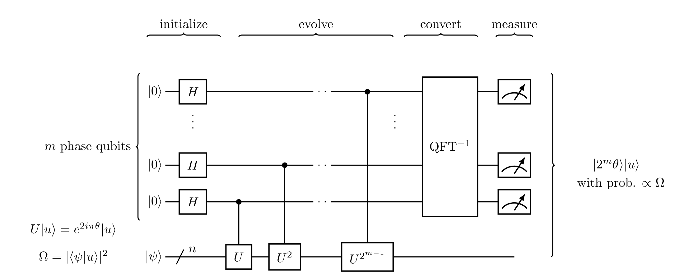
1. The physical register starts in state \(\ket{\psi}\), where \(\ket{\psi}\) is an estimate of \(\ket{u}\) with fidelity \(\Omega = \vert \langle \psi \vert u \rangle \vert^2\).

2. The phase register is initially in state \(\ket{0}\).

3. The circuit starts with a Hadamard wall to put the phase register into a superposition state.

4. Then we encode the phase into the phase register via a sequence of controlled powers of \(U\):

   \(U^{2^k}, k=0,1,...,m-1\) is applied to the physical register, conditioned on the \(k\)-th phase qubit.

5. Finally to decode the phase, we apply the inverse Quantum Fourier Transform (QFT) on the phase register.

6. We measure the phase register and find a \(m\)-bits approximation to \(\theta\) with probability \(\propto \Omega\) (at least \(4\Omega/\pi^2\), see below).

7. After the measure, the physical register has been projected onto \(\ket{u}\).

The notebook is organised as follows: In the first section, we illustrate and detail the different parts of the algorithm on a small 1D Heisenberg Hamiltonian. In the second section, we study the precision and success probability of the algorithm in more detail. Finally, in the third section we focus on the influence of the initial overlap \(\Omega\).

import time

import matplotlib.pyplot as plt
import numpy as np
from IPython.display import display
from quimb.tensor import MatrixProductState
from tqdm import notebook as tqdm

import qpe_toolbox.estimation as qpe
from qpe_toolbox import EXACT
from qpe_toolbox.circuit import make_circ
from qpe_toolbox.hamiltonian import do_dmrg, heisenberg_hamiltonian

plt.rcParams.update({"font.size": 12})

3.1. Quantum phase estimation

3.1.1. Example : 1D Heisenberg Hamiltonian

First let us define a simple Hamiltonian which we can

• diagonalize exactly

• encode as a quantum circuit

Consider the nearest-neighbor Heisenberg Hamiltonian on a 1D chain wih open boundary conditions

\[ H = J \sum_{k=0}^{L-1} \vec{S}_k \cdot \vec{S}_{k+1} \]

where \(\vec{S}_k = \vec{\sigma}_k /2 \;\) are the spin-1/2 generators of SU(2) acting on site \(k\), with \(\vec{\sigma} = (\sigma^x, \sigma^y, \sigma^z)\) the Pauli matrices.

We take \(J=1\) in the following, such that all energies are expressed in units of \(J\).

3.1.1.1. 1. Hamiltonian definition, circuit initialization

Let us define the Hamiltonian and perform exact diagonalization

n_qubits = 2
h_spin = heisenberg_hamiltonian(n_qubits)

# Get matrix
hamilt_matrix = h_spin.to_dense()

# Diagonalize hamiltonian
eigvals, eigvecs = np.linalg.eigh(hamilt_matrix)
# Ground state
E0 = eigvals[0]
psi0 = eigvecs[:, 0]
print(f"E_ED : {E0:.4f}")

E_ED : -0.7500

# Ground state MPS
E0_dmrg, psi0_mps = do_dmrg(h_spin)
print(f"E_DMRG : {E0_dmrg:.4f}")

E_DMRG : -0.7500

F = abs(psi0_mps.H @ MatrixProductState.from_dense(psi0)) ** 2
print(f"1 - |<psi_DMRG|psi_ED>|^2 = {abs(1 - F):.4g}")

1 - |<psi_DMRG|psi_ED>|^2 = 4.441e-16

We now initialize the QPE circuit with a data register containing \(|\psi_0\rangle\), and a phase register with \(m=4\) phase qubits; then measure the energy from the circuit

n_phase_bits = 4

psi_target = psi0_mps
initial_circ = make_circ(n_phase_bits, psi_target)

data_reg = list(range(n_phase_bits, n_phase_bits + n_qubits))
print(
    f"measure H = {initial_circ.local_expectation(hamilt_matrix, where=data_reg):.4f}"
)

measure H = -0.7500

3.1.1.2. First stage of Quantum Phase Estimation Algorithm

See e.g. Nielsen and Chuang.

• First, initialize the phase register with a “Hadamard wall”

• Then build the operator \(U = \exp(-i H t)\) for a given evolution time \(t\) and apply a sequence of gates ctrl-\(U^k\) on the qubit-register conditioned on the \(k\)-th phase qubit.

  Since \(|\psi_0 \rangle\) is an eigenstate of \(H\), we have \(U |\psi_0 \rangle = \exp(-i2\pi \theta) |\psi_0 \rangle\) with \(0 \leq \theta \leq 1\) (\(U\) is unitary by hermiticity of \(H\)).

  The state of the phase register is then

\[ \frac{1}{\sqrt{2^m}} \sum_{q=0}^{2^m-1} e^{i2\pi \theta q} |q \rangle ,\]

(the data register stays in the state \(|\psi_0\rangle\))

E_target = E0 + 0.2
size_interval = 2

Emax = E_target + size_interval / 2
evolution_time = 2 * np.pi / size_interval
global_phase = Emax * evolution_time

traces, circ = qpe.qpe_first_stage(
    h_spin, initial_circ, evolution_time, EXACT, global_phase
)

circ.psi.retag_({f"I{i}": f"I_phase{i}" for i in range(n_phase_bits)})
phase_reg = list(range(n_phase_bits))
psi = circ.psi.copy()
display(psi)

MatrixProductState(tensors=22, indices=31, L=6, max_bond=2)

Tensor(shape=(2), inds=[_f42d84AAAAQ], tags={I0, PSI0}),

backend=numpy, dtype=float64, data=array([1., 0.])

Tensor(shape=(2), inds=[_f42d84AAAAR], tags={I1, PSI0}),

backend=numpy, dtype=float64, data=array([1., 0.])

Tensor(shape=(2), inds=[_f42d84AAAAS], tags={I2, PSI0}),

backend=numpy, dtype=float64, data=array([1., 0.])

Tensor(shape=(2), inds=[_f42d84AAAAT], tags={I3, PSI0}),

backend=numpy, dtype=float64, data=array([1., 0.])

Tensor(shape=(2, 2), inds=[_f42d84AAAAF, _f42d84AAAAd], tags={I4, PSI0}),

backend=numpy, dtype=complex128, data=array([[0.+0.j, 1.+0.j], [1.+0.j, 0.+0.j]])

Tensor(shape=(2, 2), inds=[_f42d84AAAAF, _f42d84AAAAe], tags={I5, PSI0}),

backend=numpy, dtype=complex128, data=array([[-0.70710678+0.j, -0. +0.j], [ 0. +0.j, 0.70710678+0.j]])

Tensor(shape=(2, 2), inds=[_f42d84AAAAU, _f42d84AAAAQ], tags={GATE_0, ROUND_0, H, I0}),

backend=numpy, dtype=complex128, data=array([[ 0.70710678+0.j, 0.70710678+0.j], [ 0.70710678+0.j, -0.70710678+0.j]])

Tensor(shape=(2, 2), inds=[_f42d84AAAAf, _f42d84AAAAR], tags={GATE_1, ROUND_0, H, I1}),

backend=numpy, dtype=complex128, data=array([[ 0.70710678+0.j, 0.70710678+0.j], [ 0.70710678+0.j, -0.70710678+0.j]])

Tensor(shape=(2, 2), inds=[_f42d84AAAAq, _f42d84AAAAS], tags={GATE_2, ROUND_0, H, I2}),

backend=numpy, dtype=complex128, data=array([[ 0.70710678+0.j, 0.70710678+0.j], [ 0.70710678+0.j, -0.70710678+0.j]])

Tensor(shape=(2, 2), inds=[_f42d84AAABB, _f42d84AAAAT], tags={GATE_3, ROUND_0, H, I3}),

backend=numpy, dtype=complex128, data=array([[ 0.70710678+0.j, 0.70710678+0.j], [ 0.70710678+0.j, -0.70710678+0.j]])

Tensor(shape=(2, 2), inds=[_f42d84AAAAc, _f42d84AAAAU], tags={GATE_4, ROUND_1, PHASE, I0}),

backend=numpy, dtype=complex128, data=array([[1. +0.j , 0. +0.j ], [0. +0.j , 0.15643447+0.98768834j]])

Tensor(shape=(2, 2, 2), inds=[_f42d84AAAAb, k0, _f42d84AAAAc], tags={I0, GATE_5}),

backend=numpy, dtype=complex128, data=array([[[1.+0.j, 0.+0.j], [0.+0.j, 1.+0.j]], [[0.+0.j, 0.+0.j], [0.+0.j, 1.+0.j]]])

Tensor(shape=(2, 2, 2, 2, 2), inds=[_f42d84AAAAb, _f42d84AAAAo, _f42d84AAAAp, _f42d84AAAAd, _f42d84AAAAe], tags={I4, I5, GATE_5}),

backend=numpy, dtype=complex128, data=array([[[[[ 1. +0.00000000e+00j, 0. +0.00000000e+00j], [ 0. +0.00000000e+00j, 0. +0.00000000e+00j]], [[ 0. +0.00000000e+00j, 1. +0.00000000e+00j], [ 0. +0.00000000e+00j, 0. +0.00000000e+00j]]], [[[ 0. +0.00000000e+00j, 0. +0.00000000e+00j], [ 1. +0.00000000e+00j, 0. +0.00000000e+00j]], [[ 0. +0.00000000e+00j, 0. +0.00000000e+00j], [ 0. +0.00000000e+00j, 1. +0.00000000e+00j]]]], [[[[-0.29289322-7.07106781e-01j, 0. +0.00000000e+00j], [ 0. +0.00000000e+00j, 0. +0.00000000e+00j]], [[ 0. +0.00000000e+00j, -1. +1.46809197e-16j], [ 0.70710678-7.07106781e-01j, 0. +0.00000000e+00j]]], [[[ 0. +0.00000000e+00j, 0.70710678-7.07106781e-01j], [-1. +1.43740670e-16j, 0. +0.00000000e+00j]], [[ 0. +0.00000000e+00j, 0. +0.00000000e+00j], [ 0. +0.00000000e+00j, -0.29289322-7.07106781e-01j]]]]])

Tensor(shape=(2, 2), inds=[_f42d84AAAAn, _f42d84AAAAf], tags={GATE_6, ROUND_2, PHASE, I1}),

backend=numpy, dtype=complex128, data=array([[ 1. +0.j , 0. +0.j ], [ 0. +0.j , -0.95105652+0.30901699j]])

Tensor(shape=(2, 2, 2), inds=[_f42d84AAAAm, k1, _f42d84AAAAn], tags={I1, GATE_7}),

backend=numpy, dtype=complex128, data=array([[[1.+0.j, 0.+0.j], [0.+0.j, 1.+0.j]], [[0.+0.j, 0.+0.j], [0.+0.j, 1.+0.j]]])

Tensor(shape=(2, 2, 2, 2, 2), inds=[_f42d84AAAAm, _f42d84AAAAz, _f42d84AAABA, _f42d84AAAAo, _f42d84AAAAp], tags={I4, I5, GATE_7}),

backend=numpy, dtype=complex128, data=array([[[[[ 1.0000000e+00+0.00000000e+00j, 0.0000000e+00+0.00000000e+00j], [ 0.0000000e+00+0.00000000e+00j, 0.0000000e+00+0.00000000e+00j]], [[ 0.0000000e+00+0.00000000e+00j, 1.0000000e+00+0.00000000e+00j], [ 0.0000000e+00+0.00000000e+00j, 0.0000000e+00+0.00000000e+00j]]], [[[ 0.0000000e+00+0.00000000e+00j, 0.0000000e+00+0.00000000e+00j], [ 1.0000000e+00+0.00000000e+00j, 0.0000000e+00+0.00000000e+00j]], [[ 0.0000000e+00+0.00000000e+00j, 0.0000000e+00+0.00000000e+00j], [ 0.0000000e+00+0.00000000e+00j, 1.0000000e+00+0.00000000e+00j]]]], [[[[-1.0000000e+00-1.00000000e+00j, 0.0000000e+00+0.00000000e+00j], [ 0.0000000e+00+0.00000000e+00j, 0.0000000e+00+0.00000000e+00j]], [[ 0.0000000e+00+0.00000000e+00j, -1.0000000e+00-1.00000000e+00j], [ 3.8363611e-16+2.72634521e-17j, 0.0000000e+00+0.00000000e+00j]]], [[[ 0.0000000e+00+0.00000000e+00j, 3.8363611e-16+2.72634521e-17j], [-1.0000000e+00-1.00000000e+00j, 0.0000000e+00+0.00000000e+00j]], [[ 0.0000000e+00+0.00000000e+00j, 0.0000000e+00+0.00000000e+00j], [ 0.0000000e+00+0.00000000e+00j, -1.0000000e+00-1.00000000e+00j]]]]])

Tensor(shape=(2, 2), inds=[_f42d84AAAAy, _f42d84AAAAq], tags={GATE_8, ROUND_3, PHASE, I2}),

backend=numpy, dtype=complex128, data=array([[1. +0.j , 0. +0.j ], [0. +0.j , 0.80901699-0.58778525j]])

Tensor(shape=(2, 2, 2), inds=[_f42d84AAAAx, k2, _f42d84AAAAy], tags={I2, GATE_9}),

backend=numpy, dtype=complex128, data=array([[[1.+0.j, 0.+0.j], [0.+0.j, 1.+0.j]], [[0.+0.j, 0.+0.j], [0.+0.j, 1.+0.j]]])

Tensor(shape=(2, 2, 2, 2, 2), inds=[_f42d84AAAAx, _f42d84AAABK, _f42d84AAABL, _f42d84AAAAz, _f42d84AAABA], tags={I4, I5, GATE_9}),

backend=numpy, dtype=complex128, data=array([[[[[ 1.00000000e+00+0.00000000e+00j, 0.00000000e+00+0.00000000e+00j], [ 0.00000000e+00+0.00000000e+00j, 0.00000000e+00+0.00000000e+00j]], [[ 0.00000000e+00+0.00000000e+00j, 1.00000000e+00+0.00000000e+00j], [ 0.00000000e+00+0.00000000e+00j, 0.00000000e+00+0.00000000e+00j]]], [[[ 0.00000000e+00+0.00000000e+00j, 0.00000000e+00+0.00000000e+00j], [ 1.00000000e+00+0.00000000e+00j, 0.00000000e+00+0.00000000e+00j]], [[ 0.00000000e+00+0.00000000e+00j, 0.00000000e+00+0.00000000e+00j], [ 0.00000000e+00+0.00000000e+00j, 1.00000000e+00+0.00000000e+00j]]]], [[[[-2.00000000e+00-6.66133815e-16j, 0.00000000e+00+0.00000000e+00j], [ 0.00000000e+00+0.00000000e+00j, 0.00000000e+00+0.00000000e+00j]], [[ 0.00000000e+00+0.00000000e+00j, -2.00000000e+00+4.44089210e-16j], [ 5.45269041e-17-7.67272220e-16j, 0.00000000e+00+0.00000000e+00j]]], [[[ 0.00000000e+00+0.00000000e+00j, 5.45269041e-17-7.67272220e-16j], [-2.00000000e+00+4.44089210e-16j, 0.00000000e+00+0.00000000e+00j]], [[ 0.00000000e+00+0.00000000e+00j, 0.00000000e+00+0.00000000e+00j], [ 0.00000000e+00+0.00000000e+00j, -2.00000000e+00-6.66133815e-16j]]]]])

Tensor(shape=(2, 2), inds=[_f42d84AAABJ, _f42d84AAABB], tags={GATE_10, ROUND_4, PHASE, I3}),

backend=numpy, dtype=complex128, data=array([[1. +0.j , 0. +0.j ], [0. +0.j , 0.30901699-0.95105652j]])

Tensor(shape=(2, 2, 2), inds=[_f42d84AAABI, k3, _f42d84AAABJ], tags={I3, GATE_11}),

backend=numpy, dtype=complex128, data=array([[[1.+0.j, 0.+0.j], [0.+0.j, 1.+0.j]], [[0.+0.j, 0.+0.j], [0.+0.j, 1.+0.j]]])

Tensor(shape=(2, 2, 2, 2, 2), inds=[_f42d84AAABI, k4, k5, _f42d84AAABK, _f42d84AAABL], tags={I4, I5, GATE_11}),

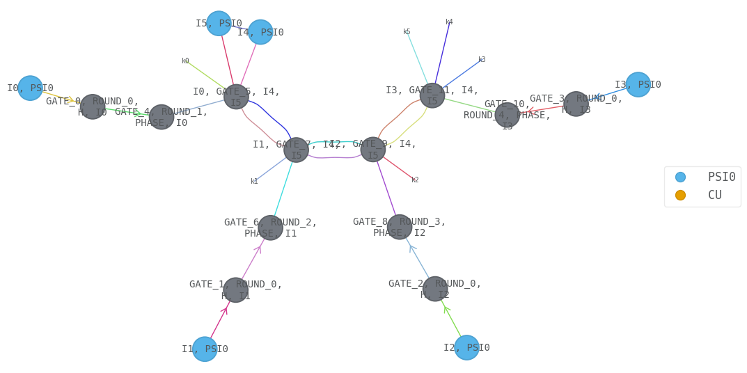
backend=numpy, dtype=complex128, data=array([[[[[ 1.00000000e+00+0.00000000e+00j, 0.00000000e+00+0.00000000e+00j], [ 0.00000000e+00+0.00000000e+00j, 0.00000000e+00+0.00000000e+00j]], [[ 0.00000000e+00+0.00000000e+00j, 1.00000000e+00+0.00000000e+00j], [ 0.00000000e+00+0.00000000e+00j, 0.00000000e+00+0.00000000e+00j]]], [[[ 0.00000000e+00+0.00000000e+00j, 0.00000000e+00+0.00000000e+00j], [ 1.00000000e+00+0.00000000e+00j, 0.00000000e+00+0.00000000e+00j]], [[ 0.00000000e+00+0.00000000e+00j, 0.00000000e+00+0.00000000e+00j], [ 0.00000000e+00+0.00000000e+00j, 1.00000000e+00+0.00000000e+00j]]]], [[[[ 8.88178420e-16+1.33226763e-15j, 0.00000000e+00+0.00000000e+00j], [ 0.00000000e+00+0.00000000e+00j, 0.00000000e+00+0.00000000e+00j]], [[ 0.00000000e+00+0.00000000e+00j, 0.00000000e+00-8.88178420e-16j], [-1.09053808e-16+1.53454444e-15j, 0.00000000e+00+0.00000000e+00j]]], [[[ 0.00000000e+00+0.00000000e+00j, -1.09053808e-16+1.53454444e-15j], [ 0.00000000e+00-8.88178420e-16j, 0.00000000e+00+0.00000000e+00j]], [[ 0.00000000e+00+0.00000000e+00j, 0.00000000e+00+0.00000000e+00j], [ 0.00000000e+00+0.00000000e+00j, 8.88178420e-16+1.33226763e-15j]]]]])

# Visualize the circuit as a tensor network
### represent controlled-U gates as a single node
for i in [n_phase_bits + 1 + 2 * j for j in range(4)]:
    psi.contract_(tags={f"GATE_{i}"})

psi.draw(
    figsize=(12, 8),
    show_tags=True,
    color={"PSI0", "CU"},
    edge_scale=1,
    layout="kamada_kawai",
    edge_color=True,
)

If we suppose that \(\theta = 0.\theta_1...\theta_m\), i.e. that \(\theta\) may exactly be expressed in \(m\) bits, then the previous expression for the state in the phase register corresponds exactly to the QFT of the product state \(|\theta_1 ... \theta_m \rangle\). Therefore, applying the inverse QFT and measuring in the computational basis gives \(\theta\) exactly. When it is not the case, the most probable output gives the closest \(m\)-bits approximation to \(\theta\).

3.1.1.3. Second stage: Inverse Quantum Fourier Transform

The state of the phase register after the inverse QFT reads:

\[ \frac{1}{2^m} \sum_{q,k=0}^{2^m-1} e^{-\frac{i2\pi}{2^m} q k}e^{i2\pi \theta q} |k \rangle .\]

Now let us introduce the following expression for \(\theta\):

\[ \theta = \frac{a}{2^m} + \delta, \]

where \(a\) is an integer between \(0\) and \(2^m-1\) and \(\delta \in [-1/2^{m+1}, 1/2^{m+1}]\). \(a/2^m\) is the best \(m\)-bit estimate of \(\theta\), and \(\delta\) a deviation from it.

The state in the phase register then reads

\[ \frac{1}{2^m} \sum_{q,k=0}^{2^m-1} e^{-\frac{i2\pi q}{2^m} (k - a)} e^{i2\pi \delta q} |k \rangle. \]

3.1.1.4. Measure and outcome

At the last step of the QPE algorithm, we sample from the phase register. We measure \(\ket{a} = \ket{[2^m \theta]}\) with probability

\[ P(a) = \left\lvert \frac{1}{2^m} \sum_{q=0}^{2^m-1} e^{i2\pi \delta q} \right\rvert^2. \]

We then see that when \(\delta=0\), then \(\theta = a / 2^m\) and \(P(a) = 1\); the outcome \(\ket{a}\) is deterministic in this case.

In the general case, \(\ket{a}\) is the most probable output with probability \(P(a) < 1\).

Let us plot this probability \(P(a)\) as a function of \(\delta\), for a given \(m\).

def prob_measure_a(delta, m):
    return (
        abs(1 / 2**m * sum([np.exp(2j * np.pi * delta * q) for q in range(2**m)])) ** 2
    )


m = 4
delta = np.linspace(-1 / 2 ** (m + 1), 1 / 2 ** (m + 1), 100)
plt.plot(delta, prob_measure_a(delta, m))
plt.title(r"Probability of measuring $|a\rangle$ when $\theta = a / 2^m + \delta$")
plt.xlabel(r"$\delta$")
plt.ylabel(r"$P(a)$");

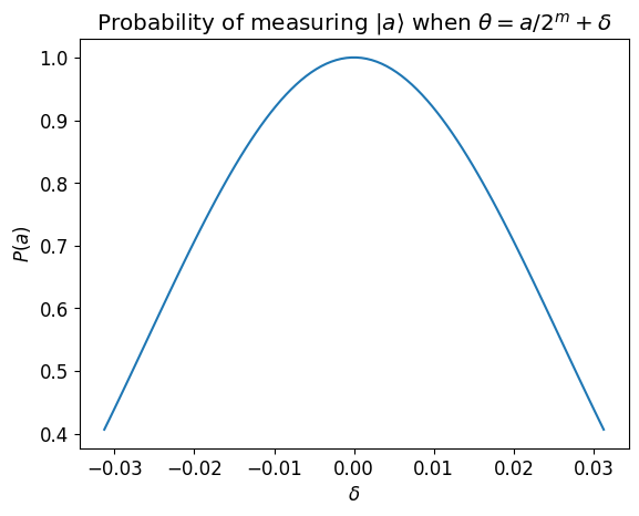
We observe that \(P(a)\) is minimal when the distance between \(\theta\) and \(a\) is maximal, i.e. for \(\delta = \pm 1/2^{m+1}\).

As shown here, there is a lower bound for the outcome probability \(P(a)\) when \(\delta \neq 0\):

\[ P(a) \geq \frac{4}{\pi^2} \simeq 0.405 \]

Below, we visualize the minimal probability \(P(a)\) for \(\delta = 1/2^{m+1}\) as a function of \(m\).

def min_prob_a(m):
    return prob_measure_a(1 / 2 ** (m + 1), m)


ms = np.arange(1, 12)
plt.plot(ms, [min_prob_a(m) for m in ms])
plt.axhline(4 / np.pi**2, color="k", linestyle=":")
plt.title(r"Probability of measuring $|a\rangle$ when $\theta = a / 2^m + 1/2^{m+1}$")
plt.xlabel(r"$m$ phase qubits")
plt.yticks([4 / np.pi**2, 0.45, 0.5], [r"$4/\pi^2$", "$0.45$", "$0.5$"])
plt.ylabel(r"$P(a)$");

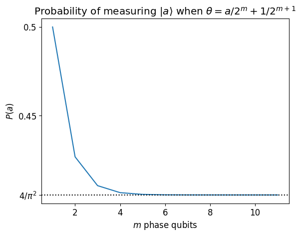
Thus with \(m\) phase qubits, we get a measure of \(\theta\) with error \(\varepsilon_\theta = 1/2^m\) with more than \(40 \%\) probability. As we will see below, adding extra qubits will increase the probability of reaching the same precision.

Note that the error and depth of the circuit is independent of the number of “physical” qubits in the data register \(n\), i.e. independent of the size of the physical system.

3.1.1.5. A note on the evolution time and global phase

\(|\psi_0 \rangle\) is an eigenstate of \(U\) with eigenvalue \(\exp(i 2\pi \theta)\) and an eigenstate of \(H\) with eigenvalue \(E_0\).

Therefore \(\exp(i2\pi\theta ) = \exp( - i E t)\); this implies

\[E t = 2\pi\theta~\mathrm{mod}~2 \pi.\]

Following the lines of the myQLM implementation of QPE, we can fix a “gauge choice” for \(\theta\) by introducing a global phase \(\phi\) in \(U\): this is done by setting \(U = \exp( - i H t + i \phi)\) and the evolution time \(t\) such that we exactly have

\[ - E t + \phi = 2 \pi \theta. \]

If we know some approximation \(E_{\rm target}\) of the exact energy \(E_0\) up to an error \(\Delta\), then by setting

\[t =2\pi/\Delta \qquad \text{and} \qquad \phi = E_{\rm max} t,\]

then

\[ E_{\rm min} \leq E_0 \leq E_{\rm max} \implies 0 \leq -E_0 t + 2\phi \leq 2\pi.\]

where \(E_{\rm max/min} = E_{\rm target} \pm \Delta/2\).

Useful expression

The correspondence between the QPE output \(\theta\) and the energy \(E\) for a given set of parameters \(E_{\rm target}\) and \(\Delta\) is

\[\theta=\frac{E_{\rm target} - E}{\Delta} + \frac{1}{2}.\]

From the previous equation, we also get an upper bound on the energy error: if we measure \(\theta\) with \(m\) bits of precision, the precision on the energy is at most \(\Delta / 2^m\).

This is a lower bound; if \(\theta\) has an exact \(m\) bits expression, the QPE algorithm will return \(E\) exactly for any number of phase qubits \(m' \geq m\).

When the initial guess is exact \(E = E_{\rm target}\), the QPE output is \(\theta = 1/2\). This case is pathological, since we precisely want to know \(E\).

3.2. Precision of exact QPE

Throughout this section, we assume that the physical register is initialized in the ground state \(\ket{\psi_0}\) and study the precision of the QPE estimate for \(E_0\).

3.2.1. An example

In this example we start with a target energy off by 0.2 : \(E_{\rm target} = E_0 + 0.2\). Let us recall that our energy scale has been fixed by defining our Hamiltonian (using \(J = 1\) in this example). Searching within an interval \(\Delta=2\), measuring \(E_0\) thus implies measuring

\[\theta=\frac{E_{\rm target} - E_0}{\Delta} + \frac{1}{2} = 0.6 .\]

To measure \(\theta\) with an error less than \(10^{-2}\) we require 5 phase qubits, since

\[(0.101)_2 = 1/2 + 1/2^3 = (0.625)_{10} ,\]

\[(0.10011)_2 = 1/2 + 1/2^4 + 1/2^5 = (0.59375)_{10} .\]

E_target = E0 + 0.2
size_interval = 2

print(f"exact theta = {(E_target + size_interval / 2 - E0) / size_interval:.6g}")

n_phase_bits = 5
print(
    f"Precision on theta = {1 / 2**n_phase_bits}, precision on energy = {1 / 2**n_phase_bits * size_interval}\n"
)

circ = make_circ(n_phase_bits=n_phase_bits, psi_mps=psi0_mps)
traces, energy = qpe.qpe_energy(
    h_spin, circ, EXACT, E_target, size_interval, verbosity=1
)

print("\nBest guess =", np.real(energy))
print("exact energy =", np.real(E0))
print("theoretical error bound =", size_interval / 2**n_phase_bits)

assert abs(E0 - energy) < size_interval / 2**n_phase_bits

exact theta = 0.6
Precision on theta = 0.03125, precision on energy = 0.0625

10011 |19> 0.59375 0.8753

10100 |20> 0.625   0.0548

10010 |18> 0.5625  0.0244

10101 |21> 0.65625 0.0109

10001 |17> 0.53125 0.0073

Best guess = -0.7375
exact energy = -0.75
theoretical error bound = 0.0625

Check that second best guess is also within an error \(\Delta / 2^m\) off the exact value

energy_bis = -size_interval * 0.625 + E_target + size_interval / 2
print("second best guess", energy_bis)
assert abs(E0 - energy_bis < size_interval / 2**n_phase_bits)

second best guess -0.8

3.2.2. Error and success probability

We have seen that when running QPE with \(m\) phase qubits, the most probable output gives an estimate of \(\theta\) with \(m\)-bits accuracy. A lower bound for this probability is \(4/\pi^2\) (recall that the physical register is initialized in the ground state \(\ket{\psi_0}\).)

In the following we investigate the probability of reaching a desired accuracy as a function of the number of phase qubits. We thus take the number of targeted bits of accuracy and the number of phase qubits to be different. Let us note \(b\) the desired number of precision bits, and \(m\) the number of phase qubits. We assume \(m \geq b\).

As stated previously, if \(\theta\) has an exact \(b\)-bits expression, then the QPE algorithm will return the exact \(\theta\) with probability \(1\) for any \(m \geq b\).

Recall that in general, for a given number \(m\) of phase qubits, \(\theta\) reads

\[ \theta = \frac{a}{2^m} + \delta, \]

where \(a\) is an integer between \(0\) and \(2^m-1\) and \(\delta \in [-1/2^{m+1}, 1/2^{m+1}]\). \(a/2^m\) is the best \(m\)-bit estimate of \(\theta\), while \(\delta\) measures the distance (or error) to this \(m\)-bit estimate. We want to estimate the probability of QPE to measure \(\theta\) with error \(\leq 1/2^b\). This is of course the case if we measure \(a\) (since \(m \geq b\)), but other outputs \(a' \in \{0, 1, ...,2^m-1\}\) may provide an estimate within \(1/2^b\) error.

We have seen that the “worst case scenario” for a given number of phase qubits \(m\) corresponds to a maximal \(\delta\), e.g.

\[ \theta = \frac{a}{2^m} + \frac{1}{2^{m+1}}. \]

Note that this “worst-case scenario” for \(m\) phase qubits corresponds to a \(\theta\) with an exact \(m+1\)-bits expression.

Suppose we want to measure \(\theta\) with \(b=4\) bits precision.

Let us take the “worst-case” scenario for \(m=b=4\), i.e.

\[ \theta = 0.5 + \frac{1}{2^5} = 0.53125. \]

One possible choice of parameters is \(E_{\rm target} = E_0 + 1/2^{m}\) and \(\Delta = 2\).

From our previous considerations, we expect that for \(m=4\) the probability of measuring \(0.5\) will be minimal and close to \(4/\pi^2\), while for \(m=5\) we expect to always measure \(\theta\) exactly; let us verify:

• First we perform QPE with \(m=4\) phase qubits

E_target = E0 + 1 / 2**4
size_interval = 2

print(f"exact theta = {(E_target + size_interval / 2 - E0) / size_interval:.6g}")

exact theta = 0.53125

n_phase_bits = 4
print(
    f"Precision on theta = {1 / 2**n_phase_bits}, precision on energy = {1 / 2**n_phase_bits * size_interval}\n"
)

circ = make_circ(n_phase_bits, psi0_mps)
traces, energy = qpe.qpe_energy(
    h_spin, circ, EXACT, E_target, size_interval, verbosity=1
)

Precision on theta = 0.0625, precision on energy = 0.125

1001 |9> 0.5625 0.4066

1000 |8> 0.5    0.4066

0111 |7> 0.4375 0.0464

1010 |10> 0.625  0.0464

0110 |6> 0.375  0.0176

prob_1 = traces["prob"]
theta_1 = traces["first_thetas"][0][0] * 1 / 2**n_phase_bits
energy_1 = -size_interval * theta_1 + E_target + size_interval / 2

print("exact energy =", E0)
print(f"size_interval / 2**(m+1) = {size_interval / 2 ** (n_phase_bits + 1)}")
print(f"\nBest guess = {energy_1} with proba {prob_1:.4f}")
print(f"error = {E0 - energy_1:.4f}")

prob_2 = traces["first_thetas"][1][1]
theta_2 = traces["first_thetas"][1][0] * 1 / 2**n_phase_bits
energy_2 = -size_interval * 0.5 + E_target + size_interval / 2
print(f"Best guess = {energy_2} with proba {prob_2:.4f}")
print(f"error = {E0 - energy_2:.4f}")

exact energy = -0.75
size_interval / 2**(m+1) = 0.0625

Best guess = -0.8125 with proba 0.4066
error = 0.0625
Best guess = -0.6875 with proba 0.4066
error = -0.0625

We find as expected two outputs with the same probability. We check that the success probability in this worst-case scenario is close to, but still above, the lower bound \(4/\pi^2 = 0.4052\).

• We now add one more phase qubit

n_phase_bits = 5
print(
    f"Precision on theta = {1 / 2**n_phase_bits}, precision on energy = {1 / 2**n_phase_bits * size_interval}\n"
)

circ = make_circ(n_phase_bits, psi0_mps)
traces, energy = qpe.qpe_energy(
    h_spin, circ, EXACT, E_target, size_interval, verbosity=1
)

Precision on theta = 0.03125, precision on energy = 0.0625

10001 |17> 0.53125 1.0000

00001 |1> 0.03125 0.0000

10011 |19> 0.59375 0.0000

01001 |9> 0.28125 0.0000

11001 |25> 0.78125 0.0000

print(f"\nBest guess = {energy} with proba {traces['prob']}")
print(f"error = {E0 - energy}")

Best guess = -0.75 with proba 1.0
error = 0.0

The output is an exact measure of \(\theta\) with probability \(1\), since \(\theta\) has an exact \(b+1=5\) bits expression.

3.2.3. General case

The goal is to measure \(\theta\) with \(b\)-bit precision. For a given “confidence level” \(1-\alpha\) (\(\alpha \in ]0,1[\)) we are looking for the minimal number of phase qubits \(m(b,\alpha) \geq b\) so that we measure \(\theta\) accurate to \(b\) bits with a probability of success at least \(1 - \alpha\). Nielsen and Chuang (section 5.2.1.) find that

\[ m(b, \alpha) = b + \left\lceil \mathrm{log}_2 \left( 2 + \frac{1}{2\alpha} \right) \right\rceil. \]

In their derivation, they take \(m > b + 1\) and introduce the best \(m\)-bits approximation to \(\theta\): \(\theta = a / 2^m + \delta,\) with \(0 < \delta < 1/2^{m+1}\).

Let the QPE output be \(r/2^m\), with \(r\) an integer in the range between \(0\) and \(2^{m-1}\). Since \(m>b\), \(r\) might be \(1/2^b\)-close to \(\theta\) even if \(r \neq a, a+1\). Indeed, one can verify that if

\[ |r - a| < 2^{m - b} - 1, \]

then

\[ \left\vert \frac{r}{2^m} - \theta \right\vert \leq \frac{1}{2^{b}}. \]

Finally, they show that the probability for QPE to measure \(\theta\) with \(b\) bits precision is

\[ 1 - P(| r - b | > 2^{m - b} - 1) > 1 - \frac{1}{2(2^{m - b} - 2)}. \]

Thus, setting \(\alpha = 1/2(2^{m - b} - 2)\), one finds that to measure \(\theta\) accurate to \(b\) bits with a probability of success at least \(1 - \alpha\), one needs a number of phase qubits

\[ m(b,\alpha) = b + \left\lceil \mathrm{log}_2 \left( 2 + \frac{1}{2\alpha} \right) \right\rceil \]

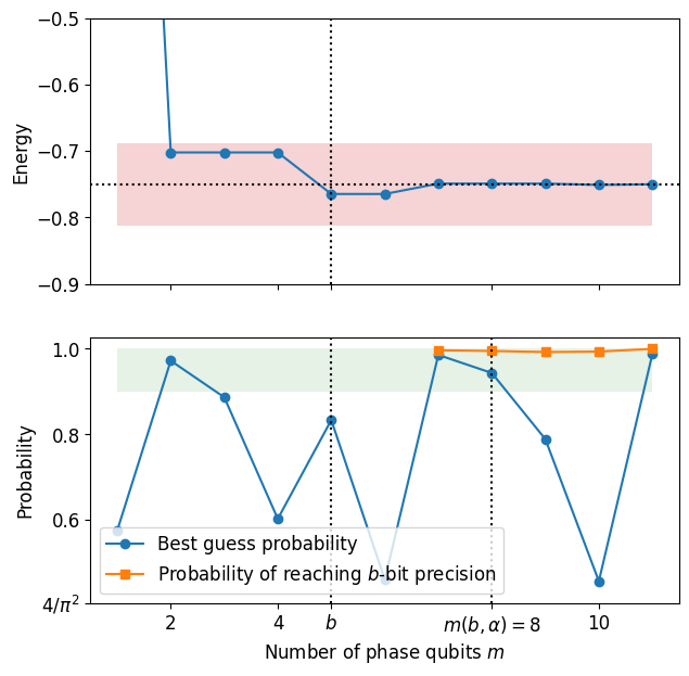
Let us now choose \(E_{\rm target} - E_0\) randomly in \([-\Delta/2,\Delta/2[\) and see how the best guess error and best guess probability evolve with \(m \geq b\).

• First we slightly modify the way we perform QPE in order to compute this probability

def qpe_with_prob_success(
    hamiltonian,
    psi0,
    theta_exact,
    n_phase_bits,
    E_target,
    size_interval,
    n_precision_bits,
):
    """
    Build the circuit and perform the quantum phase estimation algorithm.

    Return the energy, probability and probability of success as defined by Nielsen and Chuang
    """

    E_const, Emax, evolution_time, global_phase = qpe.set_search_window(
        hamiltonian, E_target, size_interval
    )

    initial_circ = make_circ(n_phase_bits, psi0)
    _, probs = qpe.qpe_sample(
        hamiltonian, initial_circ, evolution_time, EXACT, global_phase
    )

    a = np.floor(theta_exact * 2**n_phase_bits)
    prob_success = 0
    if n_precision_bits + 1 < n_phase_bits:
        for x in sorted(enumerate(np.ravel(probs)), key=lambda x: x[1], reverse=True):
            if abs(x[0] - a) < 2 ** (n_phase_bits - n_precision_bits) - 1:
                prob_success += x[1]

    max_prob_state_int = np.argmax(probs)
    theta = max_prob_state_int / 2**n_phase_bits
    energy = Emax - 2 * np.pi * theta / evolution_time + E_const
    return energy, np.max(probs), prob_success

# number of target precision bits
b = 5
# random choice for delta in [-0.5, 0.5[
rng = np.random.default_rng(seed=42)
delta = rng.random() - 1 / 2
size_interval = 2
E_target = E0 + size_interval * delta
theta_exact = (E_target + size_interval / 2 - E0) / size_interval
print(f"exact theta = {theta_exact:.6g}")

probs_success = []
probs = []
energies = []
ms = list(range(1, b + 7))

for n_phase_bits in tqdm.tqdm(ms):
    energy, prob, prob_success = qpe_with_prob_success(
        h_spin,
        psi0_mps,
        theta_exact,
        n_phase_bits,
        E_target,
        size_interval,
        n_precision_bits=b,
    )
    probs_success.append(prob_success)
    probs.append(prob)
    energies.append(energy)

exact theta = 0.773956

def minimal_number_phase_qubits(b, α):
    """Compute the minimal number of phase qubits required
    to reach b-bits precision with probability 1-α.
    """
    return b + np.ceil(np.log2(2 + 1 / (2 * α)))

fig, axs = plt.subplots(nrows=2, sharex=True, figsize=(7, 7))
axs[0].plot(ms, energies, "-o")
axs[0].axhline(y=E0, color="k", linestyle="dotted")
tol = size_interval / 2**b
axs[0].fill_between(ms, [E0 - tol], [E0 + tol], alpha=0.2, facecolor="tab:red")
axs[0].axvline(x=b, color="k", linestyle="dotted")
axs[0].set_ylabel("Energy")
axs[0].set_ylim(-0.9, -0.5)


α = 0.1
print("minimal_number_phase_qubits:", minimal_number_phase_qubits(b, α))

axs[1].plot(ms, probs, "-o", label="Best guess probability")
axs[1].plot(
    ms[b + ms[0] :],
    probs_success[b + ms[0] :],
    "-s",
    label="Probability of reaching $b$-bits precision",
)
axs[1].axvline(x=b, color="k", linestyle="dotted")
axs[1].axvline(x=minimal_number_phase_qubits(b, α), color="k", linestyle="dotted")
axs[1].fill_between(ms, [1 - α], [1], alpha=0.1, facecolor="g")
axs[1].set_ylabel("Probability")
axs[1].set_yticks([4 / np.pi**2, 0.6, 0.8, 1], [r"$4/\pi^2$", "0.6", "0.8", "1.0"])
axs[1].set_xticks([2, 4, 5, 8, 10], ["2", "4", "$b$", r"$m(b,\alpha)=8$", "10"])
axs[1].set_xlabel("Number of phase qubits $m$")
axs[1].legend(loc="lower left");

minimal_number_phase_qubits: 8.0

3.2.4. Precision versus number of phase qubits

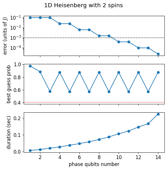
In computational chemistry, the standard level for accuracy is the so-called chemical accuracy, set to \(1\) mHa. In general, matrix elements of chemistry Hamiltonians are of the order of \(1\) Ha. In general, we will therefore aim for an error below \(\simeq 10^{-3} E_{\rm target}\). In this example we have fixed the energy unit \(J=1\), hence we shall aim for an error below or equal to \(10^{-3}\).

Assuming that we start with a first estimation of \(E_0\) with error \(0.1\), which would be the cost in the number of phase qubits to lower the error down to \(10^{-3}\)?

The answer is \(\Delta / 2^{m} \leq 10^{-3}\), i.e. \( m \geq \log_2(10^3 \Delta)\).

E_target = E0 + 0.1
size_interval = 2
print("number of phase bits for 1e-3 accuracy =", int(np.log2(10**3 * size_interval)))

number of phase bits for 1e-3 accuracy = 10

Let us see how the error decreases when increasing the number of phase qubits.

We measure the runtime of the simulation, choosing a greedy hyperoptimizer from \(\texttt{quimb}\), see our Hyperoptimization notebook for details.

optimize = "greedy"

ms = list(range(1, 15))
energies = []
probs = []
durations = []

for n_phase_bits in tqdm.tqdm(ms):
    st = time.time()
    initial_circ = make_circ(n_phase_bits, psi0_mps)
    traces, energy = qpe.qpe_energy(
        h_spin,
        initial_circ,
        EXACT,
        E_target,
        size_interval,
        optimize=optimize,
    )
    et = time.time() - st
    energies.append(energy)
    probs.append(traces["prob"])
    durations.append(traces["ctimes"][-1])

fig, axs = plt.subplots(nrows=3, sharex=True, figsize=(6, 6), layout="tight")

fig.suptitle(f"1D Heisenberg with {n_qubits} spins")
axs[0].semilogy(ms, [abs(E - E0) for E in energies], "-o")
axs[0].axhline(y=1e-3, color="k", linestyle="dotted")
axs[0].set_ylabel("error (units of J)")

axs[1].plot(ms, probs, "-o")
axs[1].axhline(y=4 / np.pi**2, color="r", linestyle="dotted")
axs[1].set_ylabel("best guess prob")

axs[2].plot(ms, durations, "-o")
axs[2].set_xlabel("phase qubits number")
axs[2].set_ylabel("duration (sec)");

3.2.5. Influence of system size (number of spins / physical qubits in the data register)

We go up to 10 spins, which corresponds to a Hilbert space of dimension \(2^{10} = 1024\), still within reach of exact diagonalization in a few seconds computation time on a laptop. The following cell may take a few minutes to run.

nqb_list = [4, 7, 10]
ms = [2, 4, 6, 8, 10]

res = {"E0": [], "energies": [], "probs": [], "durations": [], "durations_ed": []}

st0 = time.time()

for n_qubits in tqdm.tqdm(nqb_list):
    h_spin = heisenberg_hamiltonian(n_qubits)

    # Get matrix
    hamilt_qarray = h_spin.to_dense()

    # Diagonalize hamiltonian
    st_ed = time.time()
    eigvals, eigvecs = np.linalg.eigh(hamilt_qarray)
    res["durations_ed"].append(time.time() - st_ed)

    # Ground state
    E0 = eigvals[0]
    res["E0"].append(E0)
    psi0 = eigvecs[:, 0]
    psi0_mps = MatrixProductState.from_dense(psi0)
    E_target = E0 + 0.1
    size_interval = 2

    energies = []
    probs = []
    durations = []
    bond_dims = []
    for n_phase_bits in tqdm.tqdm(ms, leave=False):
        st = time.time()
        initial_circ = make_circ(n_phase_bits, psi0_mps)
        traces, energy = qpe.qpe_energy(
            h_spin, initial_circ, EXACT, E_target, size_interval, optimize=optimize
        )
        et = time.time() - st
        energies.append(energy)
        probs.append(traces["prob"])
        durations.append(traces["ctimes"][-1])

    res["energies"].append(energies)
    res["probs"].append(probs)
    res["durations"].append(durations)

for ind, n_qubits in enumerate(nqb_list):
    plt.plot(ms, res["energies"][ind], "-o", label=f"$n_{{qb}}=${n_qubits}")
plt.ylabel("Energy")
plt.xlabel("phase qubits number")
plt.legend();

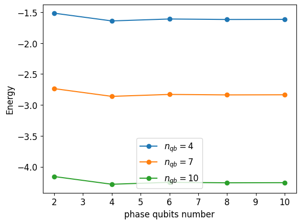
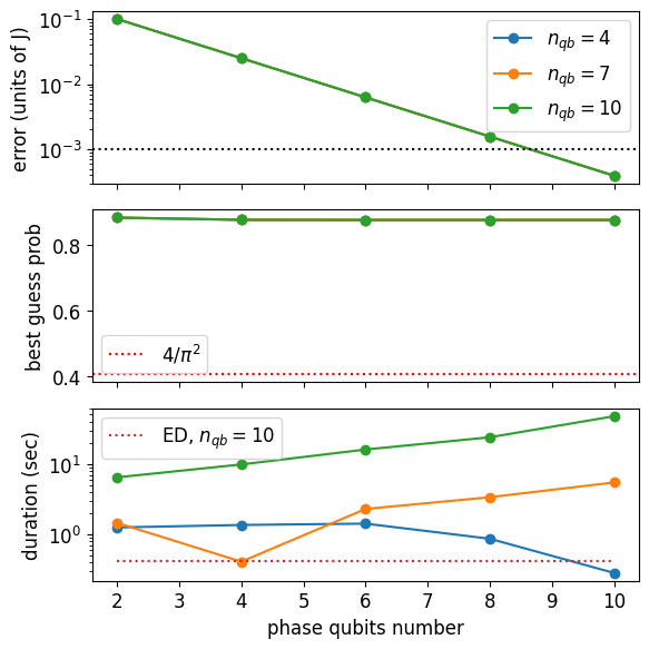
As expected, both the energy error and the success probability are independent of the number of physical qubits.

fig, axs = plt.subplots(nrows=3, figsize=(6, 6), sharex=True, layout="tight")

for ind, n_qubits in enumerate(nqb_list):
    axs[0].semilogy(
        ms,
        [abs(E - res["E0"][ind]) for E in res["energies"][ind]],
        "-o",
        label=f"$n_{{qb}}=${n_qubits}",
    )
    axs[1].plot(ms, res["probs"][ind], "-o")
    axs[2].semilogy(ms, res["durations"][ind], "-o")


axs[0].axhline(y=1e-3, color="k", linestyle="dotted")
axs[0].set_ylabel("error (units of J)")
axs[0].legend()
axs[1].axhline(y=4 / np.pi**2, color="r", linestyle="dotted", label=r"$4/\pi^2$")
axs[1].set_ylabel("best guess prob")
axs[2].semilogy(
    ms,
    [res["durations_ed"][ind] for _ in ms],
    linestyle="dotted",
    label=f"ED, $n_{{qb}}=${n_qubits}",
)
axs[2].set_xlabel("phase qubits number")
axs[2].set_ylabel("duration (sec)")
axs[2].legend()
axs[1].legend();

3.2.6. Influence of interval size and target energy

Now we try to vary the energy interval \(\Delta\) and the target energy \(E_{target}\) within an interval \([E_0 - \Delta / 2, E_0 + \Delta/2]\). Outside of this range, we are sure ti find errors after executing the algorithm, because \(\forall~k \in \mathbb{Z}\), \(\forall~\theta \in [0,1]\), \(\exp(i 2\pi \theta + i2 k \pi) = \exp(i 2\pi \theta)\).

n_qubits = 4
h_spin = heisenberg_hamiltonian(n_qubits)
E0, psi0_mps = do_dmrg(h_spin)

n_phase_bits = 10
initial_circ = make_circ(n_phase_bits, psi0_mps)

interval_sizes = np.arange(0.2 * abs(E0), 4 * abs(E0), 0.9 * abs(E0))
interval_energies = []
num_points = 11
for Δ in tqdm.tqdm(interval_sizes):
    assert Δ > 0
    energy_targets = np.linspace(E0 - 0.5 * Δ, E0 + 0.4 * Δ, num_points)
    energies_Δ = np.empty((num_points,))
    for i in tqdm.tqdm(range(num_points), leave=False):
        _, energies_Δ[i] = qpe.qpe_energy(
            h_spin, initial_circ, EXACT, energy_targets[i], Δ
        )
    interval_energies.append(energies_Δ)

fig, ax = plt.subplots()
for Δ, energies_Δ in zip(interval_sizes, interval_energies, strict=True):
    energy_targets = np.linspace(E0 - 0.5 * Δ, E0 + 0.4 * Δ, 11)
    label = rf"$\Delta={Δ / abs(E0):.2f}E_0$"
    ax.plot(energy_targets - E0, energies_Δ - E0, "-o", label=label)

ax.set_xlabel("$E_{target} - E_0$")
ax.set_ylabel("$E - E_0$")
fig.suptitle(f"{n_phase_bits} phase qubits")
ax.legend();

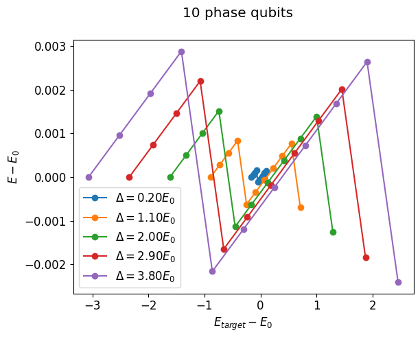
Note that the smallest the size \(\Delta\) of the search window, the smallest the error, provided \(E_0 \in [E_{\rm target}-\Delta/2, E_{\rm target}+\Delta/2]\).

3.3. Overlap

So far we had initialized the circuit with \(|\psi_0\rangle\). In practice, we don’t have a priori access to the exact \(|\psi_0\rangle\), but only an approximate state with some overlap \(\Omega\). The probability of success of QPE is then proportional to \(\Omega\).

For example, we consider the first excited state \(\ket{\psi_1}\) and initialize the physical register in state in

\[ \sqrt{\Omega} \ket{\psi_0} +\sqrt{1-\Omega} \ket{\psi_1} .\]

# Get matrix
hamilt_qarray = h_spin.to_dense()

# Diagonalize hamiltonian
eigvals, eigvecs = np.linalg.eigh(hamilt_qarray)

# Ground state
E0 = eigvals[0]
psi0 = eigvecs[:, 0]

# First excited
E1 = eigvals[1]
psi1 = eigvecs[:, 1]

size_interval = 2
E_target = E0 + 0.2  # 1 / 2**5 * size_interval

n_phase_bits = 5
Omegas = np.arange(1, -0.1, -0.1)

E_o = []
p_o = []
for Omega in Omegas:
    psi_target = np.sqrt(Omega) * psi0 + np.sqrt(1 - Omega) * psi1
    psi_target_mps = MatrixProductState.from_dense(psi_target)

    initial_circ = make_circ(n_phase_bits, psi_target_mps)
    traces_o, energy_o = qpe.qpe_energy(
        h_spin, initial_circ, EXACT, E_target, size_interval
    )
    E_o.append(energy_o)
    p_o.append(traces_o["prob"])

We plot the energy and probability outputs as a function of \(\Omega\):

fig, (ax_e, ax_p) = plt.subplots(2, 1, sharex=True)
ax_e.plot(Omegas, E_o, "-o")
ax_e.axhline(y=E0, color="k", linestyle=":", alpha=0.5)
ax_e.axhline(y=E1, color="k", linestyle=":", alpha=0.5)
ax_e.axvline(x=p_o[-1] / (p_o[0] + p_o[-1]), color="k", linestyle=":", alpha=0.5)
ax_e.set_ylabel("Energy E")
ax_e.set_yticks([E0, E1], ["$E_0$", "$E_1$"])
ax_e.xaxis.set_inverted(True)

ax_p.plot(Omegas, p_o, "-o", color="tab:orange")
ax_p.plot(Omegas, p_o[0] * Omegas, color="k", linestyle=":", alpha=0.5)
ax_p.plot(Omegas, p_o[-1] * (1 - Omegas), color="k", linestyle=":", alpha=0.5)
ax_p.axvline(x=p_o[-1] / (p_o[0] + p_o[-1]), color="k", linestyle=":", alpha=0.5)
ax_p.set_xticks(
    [0, p_o[-1] / (p_o[0] + p_o[-1]), 1], ["0", "$\\frac{p(0)}{p(0) + p(1)}$", "1"]
)
ax_p.set_ylabel("Probability p")
ax_p.set_xlabel(r"$\Omega$")
ax_p.xaxis.set_inverted(True)

fig.suptitle(
    r"QPE with initial state $\sqrt{\Omega} | \psi_0 \rangle + \sqrt{1-\Omega} | \psi_1 \rangle$"
);

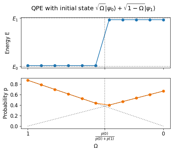
• When \(\Omega=1\) (resp. \(\Omega=0\)), the physical register is in \(\ket{\psi_0}\) (resp. \(\ket{\psi_1}\)). The energy is close but not equal to \(E_0\) (resp. \(E_1\)) and the probability is \(<1\). The energy error and finite probability depend on the number of phase qubits and on the search window parameters \(E_{\rm target}\) and \(\Delta\).

• Starting from \(\Omega=1\) and decreasing \(\Omega\), the probability decreases linearly: \(p(\Omega) = p(\Omega = 1)\Omega,\) while the energy output remains constant and close to \(E_0\). This corresponds to a decreasing overlap of the initial state with the ground state.

• There is a crossover for \(\Omega^* = p(0)/(p(0) + p(1)),\) where we switch from measuring \(E_0\) to measuring \(E_1\).

• For \(\Omega < \Omega^*\), the probability varies like: \(p(\Omega) = p(\Omega = 0) (1-\Omega),\) while the energy output remains constant and close to \(E_1\), corresponding to an increasing overlap of the initial state with the first excited state.

To go further, we encourage the reader to try starting with a state \(\sqrt{\Omega} \ket{\psi_0} + \sqrt{\frac{1-\Omega}{N-1}} \sum_{k=1}^N \ket{\psi_k}.\)