6. QPE with Linear Combination of Unitaries

In this notebook, we introduce advanced techniques for encoding the Hamiltonian into a unitary: Linear Combination of Unitaries and Qubitization. These techniques were first introduced in the context of Hamiltonian simulation and later applied to phase estimation.

We mainly take inspiration from Lin Lin’s lecture notes on Quantum Algorithms for Scientific Computation and from the paper Encoding Electronic Spectra in Quantum Circuits with Linear T Complexity, Babbush et al., PRX 8, 041015 (2018). The interested reader can read these works and references therein for the original papers where the techniques were developed.

import time

import matplotlib.pyplot as plt
import numpy as np
import quimb.tensor as qtn
from IPython.display import display
from pyscf import gto
from tqdm import notebook as tqdm

import qpe_toolbox.estimation as qpe
from qpe_toolbox.hamiltonian import (
    chemistry_hamiltonian,
    do_dmrg,
    heisenberg_hamiltonian,
)
from qpe_toolbox.tensor import apply_gate_from_mpo, kron_mps

cutoff = 1e-10
plt.rcParams.update({"font.size": 12})

• Initialization: the Linear Combination of Unitaries approach begins by rewriting the Hamiltonian into a sum of unitaries:

\[ H = \sum_{\ell=0}^{L-1} w_\ell H_\ell \qquad \mathrm{s.t.} \qquad w_\ell \geq 0, \qquad H_\ell^2 = \mathbb{1}, \]

where \(H_\ell^2 = \mathbb{1}\) expresses the condition that \(H_\ell\) is hermitian and unitary.

Spin-\(1/2\) Hamiltonians are natively written in this form since Pauli matrices are hermitian and unitary. For fermionic Hamiltonians, this decomposition can be done e.g. via the Jordan-Wigner transformation.

The weights \(w_\ell\) are defined to be positive (if needed the phase of \(w_\ell\) can always be absorbed by a re-definition of the unitary \(H_\ell\).)

We define the sum of weights, often referred to as the “1-norm” of the LCU:

\[ \lambda \equiv \sum_{\ell=0}^{L-1} w_\ell \]

Note that the cost of Quantum Phase Estimation scales with the 1-norm \(\lambda\). There is a lot of research activity devoted to compressing the Hamiltonian and reducing \(\lambda\), see e.g. this work and this more recent work and references therein. These advanced LCU techniques are beyond the scope of this simple introduction, where we consider a naive LCU based on the Pauli decomposition of \(H\).

We then introduce an empty ancilla register of size \(m_L\)

\[ m_L \equiv \lceil{ \mathrm{log}_2 (L) \rceil}\]

In the case where \(L < 2^{m_L}\) we complete the weights up to \(2^{m_L}\) by setting

\[ w_\ell = 0,~H_\ell = \mathbb{1} \qquad \mathrm{for}~ L \leq \ell < 2^{m_L}.\]

We consider the 1D Heisenberg model with 4 spins

n_qubits = 4
H = heisenberg_hamiltonian(n_qubits)

weights, λ, L, m_L = qpe.get_lcu_weights(H)
print(f"LCU decomposition with {L} terms")
print(f"Auxiliary register with {m_L} qubits")
print(f"1-norm of LCU coefficients: lambda = {λ:.3f}")

# DMRG E0 and psi0
E0_dmrg, psi0_mps = do_dmrg(H)
print(f"DMRG energy: E0 = {E0_dmrg:.3f}")

LCU decomposition with 9 terms
Auxiliary register with 4 qubits
1-norm of LCU coefficients: lambda = 2.250
DMRG energy: E0 = -1.616

The LCU scheme involves two oracles: PREPARE and SELECT, that we introduce in the following.

6.1. l-register and PREPARE oracle

The PREPARE oracle acts on the \(m_L\) qubits of the auxiliary \(\ell\)-register to prepare a superposition state related to the LCU decomposition:

\[ \mathrm{PREPARE} \equiv \sum_{\ell=0}^{L-1} \sqrt{\frac{w_\ell}{\lambda}} \ket{\ell}\bra{0} \]

The quantum circuit implementation of the PREPARE oracle relies on complicated subroutines like unary iteration and QROM (see this paper cited in introduction), that are beyond the scope of this introduction. Here, we consider a simple implementation of PREPARE as a MPO. It will be sufficient to introduce the general ideas of LCU-based qubitization.

prepare_mpo = qpe.build_lcu_prepare_mpo(H)

The state prepared by the action of the PREPARE oracle is called the \(\ket{\mathcal{L}}\) state:

\[ \mathrm{PREPARE} \ket{0}^{\otimes m_L} \mapsto \sum_{\ell=0}^{L-1} \sqrt{\frac{w_\ell}{\lambda}} \ket{\ell} \equiv \ket{\mathcal{L}} \]

zero_mps = qtn.MPS_computational_state("0" * m_L)
L_mps = prepare_mpo.apply(zero_mps)

Alernatively, the \(\ket{\mathcal{L}}\) state can be directly build calling the build_lcu_prepare_state_mps function

print(
    f"overlap (should be 1) = {L_mps.overlap(qpe.build_lcu_prepare_state_mps(H)):.3f}"
)

overlap (should be 1) = 1.000

6.2. SELECT oracle gate

Let us then introduce the second LCU oracle, the SELECT oracle. It is a unitary operation acting on both the auxiliary \(\ell\)-register and the physical register following

\[ \mathrm{SELECT}~:~ \ket{\ell}\ket{\psi} \mapsto \ket{\ell} H_\ell \ket{\psi},\]

\[ \mathrm{SELECT} \equiv \sum_{\ell=0}^{L-1} |\ell\rangle \langle \ell| \otimes H_\ell, \]

Note that for any \(\ket{\psi}\) we have:

\[ \bra{\psi}\bra{\mathcal{L}} \mathrm{SELECT} \ket{\mathcal{L}}\ket{\psi} = \bra{\psi}\frac{H}{\lambda}\ket{\psi} \]

i.e. the combination of SELECT and PREPARE gives an encoding of the Hamiltonian. This property allows to construct a unitary operator: \(\mathcal{W}\), the walk operator, that gives an exact encoding of the spectrum of \(H\) via a technique called qubitization.

select_gates = qpe.lcu_select_gates(H)

In our simple example of a spin Hamiltonian, the unitaries \(H_\ell\) are Pauli strings (\(XX, YY, ZZ\)). Note that for LCU of chemistry Hamiltonians, more advanced schemes like Single Factorization, Double Factorization, Tensor Hyper Contraction… are introduced where the unitaries \(H_\ell\) do not coincide anymore with Pauli strings (see e.g. this work on Tensor Hyper Contraction for a discussion).

print(*select_gates[:10], sep="\n")

<Gate(label=X, params=[], qubits=(0,))>
<Gate(label=X, params=[], qubits=(1,))>
<Gate(label=X, params=[], qubits=(2,))>
<Gate(label=X, params=[], qubits=(3,))>
<Gate(label=X, params=[], qubits=(4,), controls=(0, 1, 2, 3)))>
<Gate(label=X, params=[], qubits=(5,), controls=(0, 1, 2, 3)))>
<Gate(label=X, params=[], qubits=(0,))>
<Gate(label=X, params=[], qubits=(1,))>
<Gate(label=X, params=[], qubits=(2,))>
<Gate(label=X, params=[], qubits=(3,))>

The first gates correspond to \(\ket{0}\bra{0} \otimes X_0 X_1\) in “Hamiltonian” notation, where \(X_i\) represents the \(X\) Pauli matrix acting on the \(i-\)th spin of the Heisenberg model, or \(i\)-th physical qubit. Since the physical register indexing is shifted by \(m_L=4\) to avoid confusion with the auxiliary \(\ell\)-register, the first and second qubits of the physical register (index \(0\) and \(1\) in the physical register “local” indexing) correspond to qubit \(4\) and \(5\) in the total register.

We start by projecting \(\ket{0}^{\otimes m_L}\) onto \(\ket{1}^{\otimes m_L}\) (apply \(X\) on qubits \(0\) to \(3\)), then apply a controlled-\(X\) on qubit \(4\) and \(5\), then apply the reversed projection \(\ket{0}^{\otimes m_L} \bra{1}^{\otimes m_L}\).

Note that qubits in the \(\ell\)-register are indexed from \(0\) to \(m_L-1\). Qubits in the physical register are indexed from \(m_L\) to \(m_L + n - 1\).

Applying the SELECT oracle on \(\ket{\mathcal{L}}\ket{\psi_0}\), and projecting onto the same state, we get a measure of the ground state energy:

\[ \bra{\psi_0} \bra{\mathcal{L}} \mathrm{SELECT} \ket{\mathcal{L}} \ket{\psi_0} = \frac{E_0}{\lambda}. \]

Lpsi_mps = kron_mps(L_mps, psi0_mps)

circ = qtn.CircuitMPS(psi0=Lpsi_mps)
for gate in select_gates:
    circ.apply_gate(gate)

assert np.isclose(Lpsi_mps.H @ circ.psi, E0_dmrg / λ)

Proof:

\[ \mathrm{SELECT} \ket{\mathcal{L}} \ket{\psi_0} = \sum_\ell \sqrt{\frac{w_\ell}{\lambda}} \ket{\ell}H_\ell \ket{\psi_0} \]

\[ \bra{\psi_0} \bra{\mathcal{L}} \mathrm{SELECT} \ket{\mathcal{L}} \ket{\psi_0} = \sum_\ell \frac{w_\ell}{\lambda} \bra{\psi_0} H_\ell \ket{\psi_0} = \frac{1}{\lambda} \bra{\psi_0} H \ket{\psi_0} = \frac{E_0}{\lambda}\]

6.3. Walk operator

We are now ready to build the Walk operator, defined by

\[ \mathcal{W} = \mathcal{R}_L \cdot \mathrm{SELECT}, \qquad \mathcal{R}_L \equiv \left(2 \ket{\mathcal{L}} \bra{\mathcal{L}} \otimes \mathbb{1} - \mathbb{1} \right) \]

First we define \(\mathcal{R}_L\) as a MPO. Since we simulate quantum circuits as tensor networks we can always replace any part of the circuit by a MPO. In a real QPU one would need to build a Householder reflection circuit that involves a \(\mathrm{PREPARE}\) and \(\mathrm{PREPARE}^\dagger\); circuits with non trivial subroutines that are beyond the scope of this introduction.

6.3.1. Reflection as a MPO

The PREPARE oracle is key to build a reflection operator:

\[\mathcal{R}_{L} = 2 \ket{\mathcal{L}}\bra{\mathcal{L}}\otimes\mathbb{1} - \mathbb{1} \]

that will enter in the definition of the Walk operator.

Here, we build this reflection as a MPO.

R_L = qpe.build_lcu_reflection_mpo(H)
display(R_L)

MatrixProductOperator(tensors=8, indices=23, L=8, max_bond=5)

Tensor(shape=(4, 2, 2), inds=[_04cbeaAAAMM, k0, b0], tags={I0}),

backend=numpy, dtype=float64, data=array([[[ 1.04515342e+01, -1.93349009e-17], [ 4.75020052e-16, 1.04515342e+01]], [[ 3.49796120e+00, 9.99417487e-01], [ 9.99417487e-01, -3.49796120e+00]], [[-2.19781582e-01, -6.88641291e-01], [ 2.22711236e+00, 2.19781582e-01]], [[-4.00509566e-01, 2.20180052e+00], [ 6.01766449e-01, 4.00509566e-01]]])

Tensor(shape=(4, 5, 2, 2), inds=[_04cbeaAAAMM, _04cbeaAAAMN, k1, b1], tags={I1}),

backend=numpy, dtype=float64, data=array([[[[ 0.67451694, -0.06166299], [-0.06166299, 0.69468154]], [[ 0.04665332, 0.15785471], [ 0.15785471, 0.04140364]], [[ 0.00669729, -0.00669729], [-0.00669729, -0.00669729]], [[-0.01206215, 0.01206215], [ 0.01206215, 0.01206215]], [[-0.01282738, -0.00472332], [-0.00472332, 0.01192642]]], [[[-0.13789783, -0.18196886], [-0.18196886, -0.17033734]], [[ 0.49156396, 0.47106109], [ 0.47106109, 0.43605654]], [[-0.01850055, 0.03593764], [-0.03593764, -0.01850055]], [[ 0.03332039, 0.01995372], [-0.01995372, 0.03332039]], [[ 0.05878383, -0.01132176], [-0.01132176, -0.01304765]]], [[[-0.05121922, -0.0728255 ], [ 0.08957485, 0.05121922]], [[ 0.13111908, 0.24218817], [-0.24654872, -0.13111908]], [[ 0.65474678, 0.58612095], [ 0.06306285, 0.00556298]], [[ 0.00306774, -0.15256852], [ 0.16565547, -0.0100192 ]], [[-0.00392334, 0.02232919], [-0.0017679 , 0.00392334]]], [[[-0.09333715, 0.05982023], [-0.02929776, 0.09333715]], [[ 0.23893924, -0.13807151], [ 0.13012525, -0.23893924]], [[ 0.00343435, 0.1670044 ], [-0.17370752, 0.01013746]], [[-0.65497768, -0.05677494], [-0.57994467, -0.01825807]], [[-0.00714952, 0.01212279], [ 0.02534619, 0.00714952]]]])

Tensor(shape=(5, 4, 2, 2), inds=[_04cbeaAAAMN, _04cbeaAAAMO, k2, b2], tags={I2}),

backend=numpy, dtype=float64, data=array([[[[-6.89339542e-01, 6.20104652e-02], [ 6.20104652e-02, -7.08073302e-01]], [[ 6.20231399e-02, 6.13025990e-02], [ 6.13025990e-02, 6.33637224e-02]], [[-1.11266573e-02, 9.52356129e-03], [ 9.52356129e-03, 7.92046530e-03]], [[ 3.91342395e-17, 1.84636758e-03], [-1.84636758e-03, 4.06538362e-17]]], [[[ 1.29913331e-01, 4.01616694e-01], [ 4.01616694e-01, 8.52402242e-02]], [[ 4.35656780e-01, 4.02465411e-01], [ 4.02465411e-01, 3.66914958e-01]], [[ 9.43633455e-03, 1.82140176e-02], [ 1.82140176e-02, 4.58643698e-02]], [[ 6.64315954e-19, -3.18463237e-02], [ 3.18463237e-02, 6.41666445e-18]]], [[[ 1.48486040e-01, 2.33821377e-01], [-2.70942887e-01, -1.48486040e-01]], [[ 1.47339413e-01, 2.79435179e-01], [-2.84039535e-01, -1.47339413e-01]], [[-2.80865756e-01, -3.50353220e-01], [ 8.79048909e-02, -1.84174266e-02]], [[-5.04764264e-01, -3.82307417e-01], [-1.22456847e-01, 1.77775106e-17]]], [[[-2.67430640e-01, 1.73559458e-01], [-1.06701797e-01, 2.67430640e-01]], [[-2.65365508e-01, 1.60575923e-01], [-1.52283251e-01, 2.65365508e-01]], [[ 5.05852999e-01, 1.14673699e-01], [ 3.58008612e-01, 3.31706885e-02]], [[-2.80261255e-01, 9.38711827e-02], [-3.74132438e-01, -1.18111405e-18]]], [[[-2.84662848e-01, -7.96313779e-03], [-7.96313779e-03, 2.53901002e-01]], [[ 2.29543206e-01, 3.01290390e-02], [ 3.01290390e-02, -3.12147121e-01]], [[ 5.71447972e-01, -3.05233181e-01], [-3.05233181e-01, -3.90183901e-02]], [[ 2.08021574e-15, -3.06613180e-01], [ 3.06613180e-01, -1.75837019e-17]]]])

Tensor(shape=(4, 1, 2, 2), inds=[_04cbeaAAAMO, _04cbeaAAAMP, k3, b3], tags={I3}),

backend=numpy, dtype=float64, data=array([[[[-7.07106781e-01, 1.11022302e-16], [-8.84708973e-17, -7.07106781e-01]]], [[[-8.77058019e-02, -7.01646415e-01], [-7.01646415e-01, 8.77058019e-02]]], [[[ 7.01646415e-01, -8.77058019e-02], [-8.77058019e-02, -7.01646415e-01]]], [[[-0.00000000e+00, 7.07106781e-01], [-7.07106781e-01, -2.22044605e-16]]]])

Tensor(shape=(1, 1, 2, 2), inds=[_04cbeaAAAMP, _04cbeaAAAMQ, k4, b4], tags={I4}),

backend=numpy, dtype=float64, data=array([[[[0.70710678, 0. ], [0. , 0.70710678]]]])

Tensor(shape=(1, 1, 2, 2), inds=[_04cbeaAAAMQ, _04cbeaAAAMR, k5, b5], tags={I5}),

backend=numpy, dtype=float64, data=array([[[[0.70710678, 0. ], [0. , 0.70710678]]]])

Tensor(shape=(1, 1, 2, 2), inds=[_04cbeaAAAMR, _04cbeaAAAMS, k6, b6], tags={I6}),

backend=numpy, dtype=float64, data=array([[[[0.70710678, 0. ], [0. , 0.70710678]]]])

Tensor(shape=(1, 2, 2), inds=[_04cbeaAAAMS, k7, b7], tags={I7}),

backend=numpy, dtype=float64, data=array([[[-0.70710678, 0. ], [ 0. , -0.70710678]]])

6.3.2. Walk operator

Let us apply SELECT on the \(\ket{\mathcal{L}}\ket{\psi}\) state

circ = qtn.CircuitMPS(psi0=Lpsi_mps)

select_gates = qpe.lcu_select_gates(H)
for gate in select_gates:
    circ.apply_gate(gate)

select_Lpsi = circ.psi

For an eigenstate \(\ket{\psi_k}\) with eigenvalue \(E_k\), the action of \(\mathcal{W}\) on \(\ket{\mathcal{L}}\ket{\psi_k}\) spans a two-dimensional space defined by \(\ket{\psi_k}\) and an orthogonal state \(\ket{\phi_k}\)

\[ \mathrm{SELECT} \ket{\mathcal{L}}\ket{\psi_k} = \frac{E_k}{\lambda} \ket{\mathcal{L}}\ket{\psi} + \sqrt{1-(\frac{E_k}{\lambda})^2} \ket{\phi_k}, \]

where \(\ket{\phi_k}\) is:

\[ \ket{\phi_k} = \frac{(\mathbb{1} - \ket{\mathcal{L}}\ket{\psi_k}\bra{\psi_k}\bra{\mathcal{L}}) \cdot \mathrm{SELECT} \ket{\mathcal{L}}\ket{\psi_k}}{||(\mathbb{1} - \ket{\mathcal{L}}\ket{\psi_k}\bra{\psi_k}\bra{\mathcal{L}}) \cdot \mathrm{SELECT} \ket{\mathcal{L}}\ket{\psi_k}||}. \]

By definition of \(\ket{\phi_k}\), we have \(\bra{\psi_k}\bra{\mathcal{L}} \ket{\phi_k} = 0.\)

phi = (select_Lpsi - E0_dmrg / λ * Lpsi_mps) / np.sqrt(1 - (E0_dmrg / λ) ** 2)
assert np.isclose(abs(phi.H @ Lpsi_mps) ** 2, 0)

Now let us apply the reflection \(\mathcal{R}_L\) to get \(\mathcal{W}\).

\(\mathcal{W}\) has the following matrix elements:

\[ \bra{\psi_k}\bra{\mathcal{L}} \mathcal{W} \ket{\mathcal{L}}\ket{\psi_k} = \frac{E_k}{\lambda} \]

and

\[ \bra{\phi_k} \mathcal{W} \ket{\mathcal{L}}\ket{\psi_k} = - \sqrt{1 - (\frac{E_k}{\lambda})^2} \]

circ_final = apply_gate_from_mpo(circ=circ, mpo=R_L)
psi_final = circ_final.psi.copy()

assert np.isclose(Lpsi_mps.H @ psi_final, E0_dmrg / λ)
assert np.isclose(phi.H @ psi_final, -np.sqrt(1 - (E0_dmrg / λ) ** 2))

In the basis \(\{ \ket{\mathcal{L}}\ket{\psi_k}, \ket{\phi_k} \}\), the Walk operator reads

\[ \mathcal{W} = e^{i \arccos\left({E_k/\lambda}\right) Y} \]

where we have introduced the \(Y\) Pauli matrix.

Proof: let us define

\[ \ket{\pm} = \frac{1}{\sqrt{2}} \left( \ket{\mathcal{L}}\ket{\psi_k} \pm i \ket{\phi_k} \right). \]

plus_state = 1 / np.sqrt(2) * (Lpsi_mps + 1j * phi)
minus_state = 1 / np.sqrt(2) * (Lpsi_mps - 1j * phi)

and check that

\[ \bra{\pm} \mathcal{W} \ket{\mathcal{L}}\ket{\psi_k} = \frac{\mathrm{e}^{ \pm i \arccos\left({E_k/\lambda}\right) }}{\sqrt{2}} \]

assert np.isclose(
    plus_state.H @ psi_final, np.exp(1j * np.arccos(E0_dmrg / λ)) / np.sqrt(2)
)
assert np.isclose(
    minus_state.H @ psi_final, np.exp(-1j * np.arccos(E0_dmrg / λ)) / np.sqrt(2)
)

Thus, the action of \(\mathcal{W}\) on \(\ket{\mathcal{L}}\ket{\psi_k}\) spans a two-dimensional space in which its eigenphases are exact functions of the energy \(E_k\). We can therefore apply the QPE algorithm on \(\mathcal{W}\) to find \(E_k\).

6.4. QPE on Walk operator

The run_qpe_lcu_walk_operator function from the estimation module builds the Walk operator using the different functions we have previously introduced and runs the “textbook” QPE circuit on \(\mathcal{W}\).

n_phase_qubits = 4
traces, theta = qpe.run_qpe_lcu_walk_operator(H, psi0_mps, n_phase_qubits, verbosity=1)

binary      	 ket    	 phase  	 prob
0110         	 |6>      	 0.3750 	 0.4974
1010         	 |10>     	 0.6250 	 0.4974
0111         	 |7>      	 0.4375 	 0.0010

Now we compute the energy from the eigenphase of \(\mathcal{W}\):

\[ 2 \pi \theta = \pm \arccos(E_0/\lambda) \implies E_0 = \cos(2 \pi \theta) * \lambda \]

energy = qpe.get_energy_from_lcu_walk_phase(theta, λ)
print(f"energy = {energy:.4f}")

energy = -1.5910

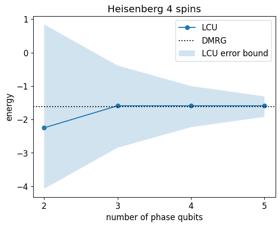
The QPE circuit returns a measure of \(\theta\) with precision of order \(\Delta\theta = 1/2^{m}\) where \(m\) is the number of phase qubits (in reality you need a little bit more than \(m\) phase qubits to reach this precision with guarantees, see the tutorial on Texbook QPE.) The precision on \(E\) is then

\[ \Delta E = \lambda \frac{2\pi}{2^m} \sqrt{1 - \left(\frac{E_0}{\lambda}\right)^2} \]

print(f"error = {abs(E0_dmrg - energy):.4f}")
delta_e = qpe.estimate_lcu_error(n_phase_qubits, E0_dmrg, λ)
print(f"error bound = {delta_e:.4f}")

error = 0.0250
error bound = 0.6148

Let us now vary the number of phase qubits

thetas = []
n_phase_bits_list = list(range(2, 6))
durations = []
energies = []
for m_ph in tqdm.tqdm(n_phase_bits_list):
    st = time.time()
    traces, theta = qpe.run_qpe_lcu_walk_operator(H, psi0_mps, m_ph)
    thetas.append(theta)
    durations.append(time.time() - st)
    energies.append(qpe.get_energy_from_lcu_walk_phase(theta, λ))

We plot the energy as a function of the number of phase qubits to see how the precision evolves

delta_es = [qpe.estimate_lcu_error(m_ph, E0_dmrg, λ) for m_ph in n_phase_bits_list]

plt.plot(n_phase_bits_list, energies, "-o", label="QPE")
plt.axhline(y=E0_dmrg, color="k", linestyle=":", label="DMRG")
plt.fill_between(
    n_phase_bits_list,
    [E0_dmrg + delta_e for delta_e in delta_es],
    [E0_dmrg - delta_e for delta_e in delta_es],
    alpha=0.2,
    label="error bound",
)
plt.legend()
plt.title(f"Heisenberg {H.n_qubits} spins - LCU")
plt.ylabel("energy")
plt.xlabel("number of phase qubits");

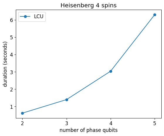
plt.plot(n_phase_bits_list, durations, "-o")
plt.ylabel("duration (seconds)")
plt.xlabel("number of phase qubits");

6.5. Compare with second order Trotter

Let’s compare with QPE applied on a Trotter approximation of the time-evolution operator.

res_ttr = {"durations": [], "energies": []}
E_target = E0_dmrg + 0.2
size_interval = 2.0
trotter_order = 2
n_steps = 6

for m_ph in tqdm.tqdm(n_phase_bits_list):
    zeros_mph = qtn.MPS_computational_state("0" * m_ph)
    psi_init = kron_mps(zeros_mph, psi0_mps)
    init_circ = qtn.CircuitMPS(psi0=psi_init, cutoff=cutoff)
    traces, energy = qpe.qpe_energy(
        H, init_circ, n_steps, E_target, size_interval, trotter_order=trotter_order
    )
    res_ttr["durations"].append(traces["ctimes"][-1])
    res_ttr["energies"].append(energy)

We visualize the convergence of the energy with the number of phase qubits

plt.plot(n_phase_bits_list, res_ttr["energies"], "-s")
plt.axhline(y=E0_dmrg, color="k", linestyle=":", label="DMRG")
plt.fill_between(
    n_phase_bits_list,
    [E0_dmrg + size_interval / 2**m_ph for m_ph in n_phase_bits_list],
    [E0_dmrg - size_interval / 2**m_ph for m_ph in n_phase_bits_list],
    alpha=0.2,
    label="error bound",
)
plt.legend()
plt.title(f"Heisenberg {H.n_qubits} spins - 2nd order Trotter {n_steps} steps")
plt.ylabel("energy")
plt.xlabel("number of phase qubits");

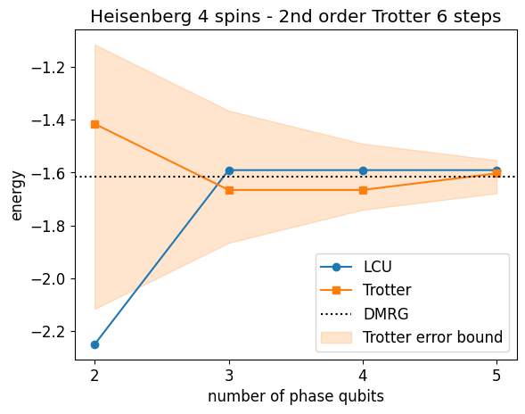
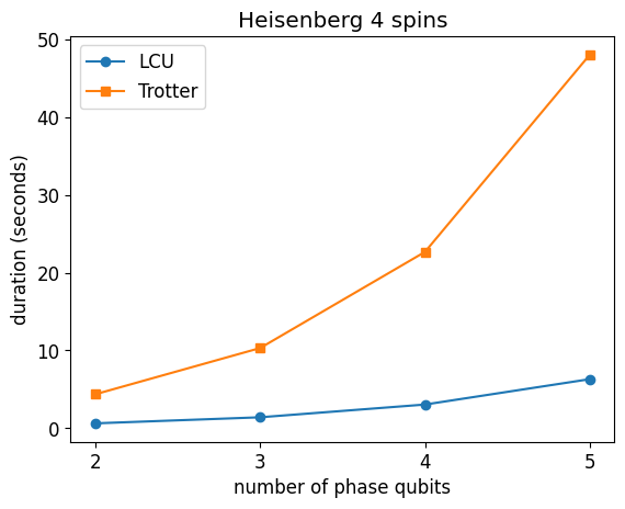
The computation is much longer, although the comparison is not completely fair. Indeed, in the LCU-based QPE we apply the REFLECT oracle as a MPO, which translates into much less gates to apply and less operations in the simulation (here the simulation time is mainly due to the number of operations, since we work with small systems the bond dimension remains small).

plt.plot(n_phase_bits_list, res_ttr["durations"], "-s")
plt.ylabel("duration (seconds)")
plt.xlabel("number of phase qubits");

6.6. Quantum chemistry example: diatomic Hydrogen

As an illustration of the use of QPE in quantum chemistry, we apply LCU to the molecular Hamiltonian describing H\(_2\) in the minimal atomic orbital basis:

mol = gto.M(
    atom=[("H", (0.0, 0.0, 0.0)), ("H", (0.0, 0.0, 0.735))],
    basis="STO-3G",
)

H_H2 = chemistry_hamiltonian(
    mol, hf_mode="rhf", encoding="original", do_fci=True, do_ccsd=False
)

converged SCF energy = -1.116998996754

nOrb   : 2
nElec  : 2
E_HF   : -1.1169989968

E_CI   : -1.1373060358

# LCU weights and related figures
weights_H2, λ_H2, L_H2, mL_H2 = qpe.get_lcu_weights(H_H2)
# DMRG energy and state
E0_H2, psi0_H2 = do_dmrg(H_H2)

print(f"E_DMRG : {E0_H2 + H_H2.e_const:.10f}")
print(f"L={L_H2} terms in the LCU decomposition \nLCU 1-norm λ = {λ_H2:.4f}")

E_DMRG : -1.1373060358
L=14 terms in the LCU decomposition 
LCU 1-norm λ = 1.8945

m_ph = 4  # number of phase qubits

# QPE on Walk operator
traces, theta = qpe.run_qpe_lcu_walk_operator(H_H2, psi0_H2, m_ph, verbosity=1)
# Get the energy
energy = qpe.get_energy_from_lcu_walk_phase(theta, λ_H2)
print(f"\nenergy = {energy:.4f}, error={abs(E0_H2 - energy):.4f}")
# Check error bound
delta_e = qpe.estimate_lcu_error(m_ph, E0_H2, λ_H2)
print(f"error bound = {delta_e:.4f}")

binary      	 ket    	 phase  	 prob
0101         	 |5>      	 0.3125 	 0.2134
1011         	 |11>     	 0.6875 	 0.2134
0110         	 |6>      	 0.3750 	 0.1990

energy = -0.7250, error=0.3217
error bound = 0.6201

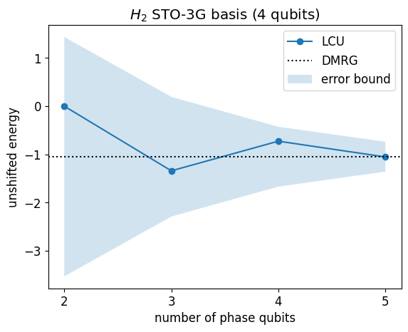
Let us plot the energy for growing number of phase qubits

thetas = []
n_phase_bits_list = list(range(2, 6))
durations = []
energies = []
for m_ph in tqdm.tqdm(n_phase_bits_list):
    st = time.time()
    traces, theta = qpe.run_qpe_lcu_walk_operator(H_H2, psi0_H2, m_ph)
    thetas.append(theta)
    durations.append(time.time() - st)
    energies.append(qpe.get_energy_from_lcu_walk_phase(theta, λ_H2))

delta_es = [qpe.estimate_lcu_error(m_ph, E0_H2, λ_H2) for m_ph in n_phase_bits_list]

plt.plot(n_phase_bits_list, energies, "-o", label="QPE")
plt.axhline(y=E0_H2, color="k", linestyle=":", label="DMRG")
plt.fill_between(
    n_phase_bits_list,
    [E0_H2 + delta_e for delta_e in delta_es],
    [E0_H2 - delta_e for delta_e in delta_es],
    alpha=0.2,
    label="error bound",
)
plt.legend()
plt.title(f"H2 STO-3 basis ({H_H2.n_qubits} qubits) - LCU")
plt.ylabel("energy")
plt.xlabel("number of phase qubits");

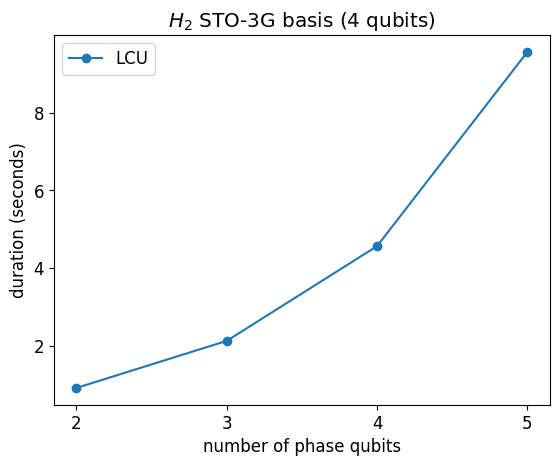
plt.plot(n_phase_bits_list, durations, "-o")
plt.ylabel("duration (seconds)")
plt.xlabel("number of phase qubits");