9. Hyperoptimization

We aim at providing more advanced circuit simulations for the toolbox; this tutorial complements the MPS contraction from a boundary of the network presented in the tutorial on MPS contraction, and focuses on how to use hyperoptimization without intermediate compression. It is used for the exact contraction of relatively large networks representing expectation values of local observables, which can contribute for example in the computation of global energy expectation values.

The particular example we chose is the optimization of the Ansatz circuit for the Quantum Approximate Optimization Algorithm (QAOA) in order to solve a MaxCut problem. This notebook is based on the several examples from \(\texttt{cotengra}\) and \(\texttt{quimb}\) for optimized contractions. In particular, we revisit the example on Bayesian Optimizing QAOA Circuit Energy.

import os

os.environ["NUMBA_NUM_THREADS"] = "1"
os.environ["OMP_NUM_THREADS"] = "1"
os.environ["MKL_NUM_THREADS"] = "1"

import cotengra as ctg
import matplotlib.pyplot as plt
import networkx as nx
import numpy as np
import quimb as qu
import quimb.tensor as qtn
from tqdm import tqdm

from qpe_toolbox.circuit import (
    brute_force_maxcut,
    draw_layered_circuit,
    draw_layered_expval,
    study_optimization_time_costs,
)

my_markers = [
    {
        "linestyle": "",
        "marker": "o",
        "markeredgecolor": "k",
        "markersize": 8,
        "markerfacecolor": "r",
    },
    {
        "linestyle": "",
        "marker": "s",
        "markeredgecolor": "k",
        "markersize": 8,
        "markerfacecolor": "gold",
    },
    {
        "linestyle": "",
        "marker": "^",
        "markeredgecolor": "k",
        "markersize": 8,
        "markerfacecolor": "limegreen",
    },
]

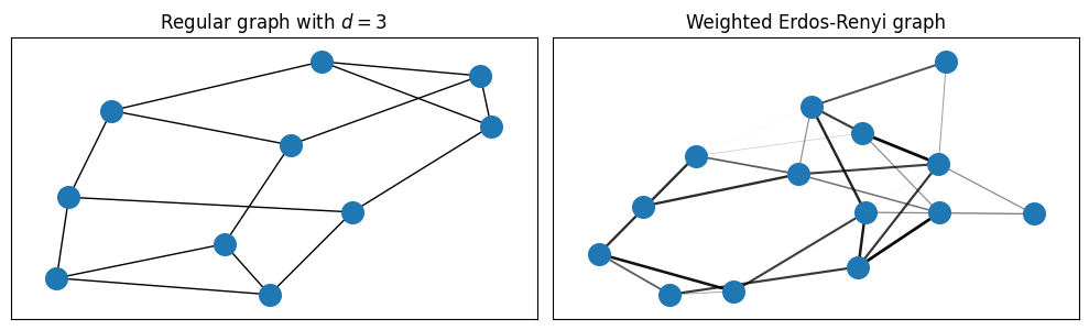
In order to present the different options for the optimized contraction, we use two different types of underlying graphs on the MaxCut problem.

rng = np.random.default_rng(42)

# random regular graph
regularity = 3
G_reg = nx.random_regular_graph(d=regularity, n=10, seed=42)
terms_reg = dict.fromkeys(G_reg.edges, 1)

# weighted Erdos-Renyi graph
graph_sparsity = 0.25
G_wER = nx.fast_gnp_random_graph(n=14, p=graph_sparsity, seed=42)
terms_wER = {(i, j): rng.random() for i, j in G_wER.edges}
amplitudes_wER = np.fromiter(terms_wER.values(), float)

For clarity, we visualize the two types of graphs. For simpler visualization of the connections, we scale the opacity of the edges by their weight.

Clearly, the random regular graph only displays three connections per node, while the Erdos-Renyi graph may include many (inequivalent) more edges.

fig, (ax_reg, ax_wER) = plt.subplots(1, 2, figsize=(10, 5 / 1.61), layout="tight")

# regular graph
positions = nx.spring_layout(G_reg, seed=42)
nx.draw_networkx_nodes(G_reg, positions, node_size=200, ax=ax_reg)
nx.draw_networkx_edges(G_reg, positions, ax=ax_reg)

# weighted Erdos-Renyi
positions = nx.spring_layout(G_wER, seed=42)
nx.draw_networkx_nodes(G_wER, positions, node_size=200, ax=ax_wER)
nx.draw_networkx_edges(
    G_wER, positions, width=2 * amplitudes_wER, alpha=amplitudes_wER, ax=ax_wER
)
ax_reg.set_title(r"Regular graph with $d=3$")
ax_wER.set_title(r"Weighted Erdos-Renyi graph")

Text(0.5, 1.0, 'Weighted Erdos-Renyi graph')

We will try to understand how complex is it to find good QAOA circuit parametrizations for each case, taking into account connectivity and the inequivalence of edges in the second case.

9.1. Building the QAOA circuits

Solving the MaxCut problem consists in finding a partition of a graph with a maximum weight across the cut

(where \(\mathrm{cut}\) is a subset of the full edge set \(E\)):

\[\mathrm{argmax}_\mathrm{cut}\Big ( \mathrm{cost_{cut}}=\sum_{(i,j) \in \mathrm{cut}} w_{ij} \Big )\]

This corresponds to finding the ground state of the classical antiferromagnetic Ising model

\[H=\sum_{(i,j)\in E} w_{ij}(1-\sigma^z_i\sigma^z_j)\]

In order to find the partition(s) with the lowest energy, the QAOA Ansatz of depth \(p\) takes inspiration from the quantum annealing approach and uses a parametrized circuit constituted by ‘Trotterized’ layers of real time evolution (see our example trotter_decomposition). It alternates the action of a mixer Hamiltonian with an easy ground state, the transverse magnetization \(\mathbb{M}_x=\sum_i \sigma^x_i\) with phase \(\beta\), and the target antiferromagnetic Ising Hamiltonian with phase \(\gamma\):

\[|\Psi_{\mathrm{Ansatz}}\rangle = U_x^{(p)}U_{zz}^{(p)}...U_x^{(1)}U_{zz}^{(1)}|\mathrm{GS}\{\mathbb{M}_x\}\rangle =e^{-i\beta_p \mathbb{M}_x} e^{-i\gamma_p H}...e^{-i\beta_1 \mathbb{M}_x} e^{-i\gamma_1 H} |\mathrm{GS}\{\mathbb{M}_x\}\rangle\]

Given the local structure of \(\mathbb{M}_x\) and \(H\) together with the ‘Trotterized’ construction of the circuit, the computation of the expectation value of the energy

\[\langle H \rangle=\sum_{(i,j)\in E} w_{ij}(1- \langle \sigma^z_i\sigma^z_j \rangle )\]

simplifies into a sum of smaller circuits \(\langle \sigma^z_i\sigma^z_j \rangle=\langle \sigma^z_i\sigma^z_j \rangle_{(i,j) ~\mathrm{causal}}\). This simplification can be further understood in the following cells; importantly, the causal networks are notably smaller and can be contracted exactly for middle-sized instances, and approximately for bigger ones.

# circuit depth
p = 3
gammas = rng.standard_normal(p)
betas = rng.standard_normal(p)

# quimb already includes constructor functions for generating the `Circuit` instance for QAOA
circ_reg = qtn.circ_qaoa(terms_reg, p, gammas, betas)
circ_wER = qtn.circ_qaoa(terms_wER, p, gammas, betas)

The constructed circuit associated to the Ansatz is the following:

fig = draw_layered_circuit(
    circ=circ_reg,
    list_names=[
        r"$0$",
        [f"$\\mathrm{{R_x^{{({i})}} }}$" for i in range(1, p + 1)],
        [r"$\mathrm{CNOT}$"] * p,
    ],
);

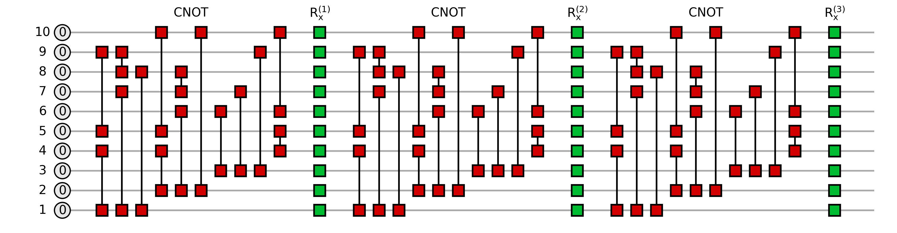
For efficiency, we may only contract the subset of gates involved in the computation of the energy of an edge, which may be much smaller thanks to the locality of the associated operator. The simplification arises from unitary cancellation

\[U U^\dagger=U^\dagger U = 1\]

and it is conditioned by the layout of the circuit: if the circuit is deep and narrow, unitary cancellation may occur only on the first layers close to the edge operator (central columns around \(h_{ij}\) in the following plot); on the other hand, the wider the circuit is, the more cancellation may occur.

The following function depicts the expectation value with unitary cancellation for the energy term between nodes 0 and 1 in the random regular graph QAOA Ansatz of depth \(p=3\). The drawing must be read from left to right as

\[\langle \mathrm{GS}\{\mathbb{M}_x\} |~ U_x^{(1)}~U_{zz}^{(1)}~U_x^{(2)}~U_{zz}^{(2)}~U_x^{(3)}~U_{zz}^{(3)}~ h_{0,1} ~U_x^{(3)}~U_{zz}^{(3)}~U_x^{(2)}~U_{zz}^{(2)}~U_x^{(1)}~U_{zz}^{(1)}~|\mathrm{GS}\{\mathbb{M}_x\}\rangle\]

with \(h_{0,1}=\sigma^z_0\sigma^z_1\).

list_names = [
    r"$+$",
    [f"$\\mathrm{{R_x^{{({i})}} }}$" for i in range(1, p + 1)],
    ["$\\mathrm{{R_{{zz}} }}$"] * p,
]
fig = draw_layered_expval(selected_edge=(3, 4), circ=circ_reg, list_names=list_names);

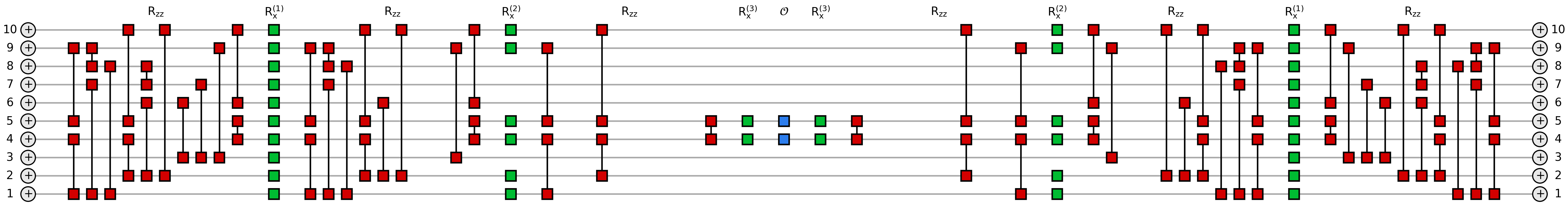
If we compare the former two pictures, we clearly see that in the expectation value the rotations of the first layer \(U^{(1)}\) (outermost, closest to the state at the edges) appear completely unchanged, while the second layer \(U^{(2)}\) is shallower thank to some cancellation, and the third layer \(U^{(3)}\) (innermost, closest to the edge operator) is more simplified.

The cost function for solving MaxCut with the QAOA Ansatz implies contracting these reduced networks for each edge observable featuring in the Hamiltonian.

The next step consists in finding the best order of contraction (which may be non trivial due to the long-range gates and the lack of periodicity). This order can be found with or without intermediate compressions. In this notebook we restrain ourselves to exact contractions.

9.2. Understanding the cost of contractions: the contraction tree, W and C

Luckily, \(\texttt{cotengra}\) automatizes the optimization process for finding the best series of pairwise contractions in a network. The whole machinery is wrapped up into a HyperOptimizer object.

When a set of contractions is to be done, hyperoptimization rehearses the contraction without really contracting the network: instead, it uses a series of registed methods for finding the best contraction path given the network and the dimensions of the tensors.

Before examining the inner workings of hyperoptimization, we first introduce the concept of a contraction tree, which is closely tied to the cost functions the hyperoptimizer seeks to minimize. For the sake of clearness, the reader may execute the following two cells (where we define generic simple hyperoptimizers and rehearse the energy computation) and jump to the next explanation.

# generic minimal options for hyperoptimization
opt_eco_reg = ctg.ReusableHyperOptimizer(
    max_repeats=128,
    methods=["greedy"],
    optlib="random",
    minimize="write",
)

opt_eco_wER = ctg.ReusableHyperOptimizer(
    max_repeats=128,
    methods=["greedy"],
    optlib="random",
    minimize="write",
)

# edge operator
ZZ = qu.pauli("Z") & qu.pauli("Z")

# rehearse the random regular graph energy
local_exp_rehs_reg = [
    circ_reg.local_expectation_rehearse(weight * ZZ, edge, optimize=opt_eco_reg)
    for edge, weight in tqdm(list(terms_reg.items()))
]

# rehearse the weighted Erdos-Renyi graph energy
local_exp_rehs_wER = [
    circ_wER.local_expectation_rehearse(weight * ZZ, edge, optimize=opt_eco_wER)
    for edge, weight in tqdm(list(terms_wER.items()))
]

The contraction tree is a representation of the contraction path together with the underlying (hyper)graph structure. It consists on the series of pairwise contractions between the tensors of the network, yielding a binary tree where the initial tensors are the leaves, and the final tensor (a scalar in our example) is in the root.

A tent representation of this contraction tree contains valuable information: the left colorbar represents the \(\log_2\) of intermediate sizes of tensors generated along the contraction sequence, corresponding to the colors of the edges in the tent tree; the maximum of these is the contraction width \(W\), thus an estimation of the RAM footprint. On the right side, the colorbar corresponds to the \(\log_{10}\) of the total number of scalar multiplications required to perform a particular contraction, corresponding to the colors of the nodes; the sum of all these is the contraction cost \(C\).

tree_reg, W, C = (
    local_exp_rehs_reg[0]["tree"],
    local_exp_rehs_reg[0]["W"],
    local_exp_rehs_reg[0]["C"],
)
print(f"W={W}, C={C}")
tree_reg.plot_tent(order=True)
tree_reg.plot_contractions();

W=11.0, C=4.67694953936863

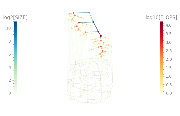
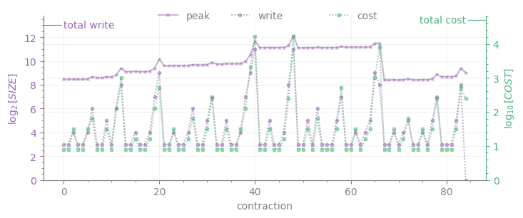
As it can be clearly seen, \(W\) coincides with the top of the left colorbar in the tent plot, while \(C\) cannot be easily read from the tent plot.

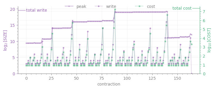
The lower plot displays the intermediate sizes for each contraction numbered by the order of execution in the tree (write, purple line with dot markers), whose maximum is \(W\); peak is the memory required for all intermediates to be stored at once (purple line with cross markers). Together with write, the cost of each contraction appears in green; the cost of the sum of all contractions (i.e. \(C\)) is displayed as a tick on the upper right corner.

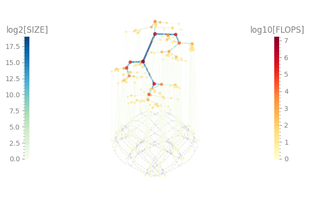
In comparison to the tree sample from the random regular graph, the trees contributing on the expectation value of the energy for the Erdos-Renyi graph may be more complex due to the higher degree of connectivity of the nodes:

tree_wER = local_exp_rehs_wER[0]["tree"]
tree_wER.plot_tent(order=True)
tree_wER.plot_contractions();

Finally, if we are interested on a global view of the required contractions for the graph, we can plot \(W\) and \(C\) for all the trees, each associated to the local expectation value of an edge operator (the x-axis correspongs to the numbering of each expectation value as it appears on the list for computing the full energy):

fig, ax = plt.subplots(nrows=2, ncols=2, figsize=(10, 10 / 1.61))

ax[0, 0].plot([rehs["W"] for rehs in local_exp_rehs_reg])
ax[0, 0].set_ylabel("contr. width, $W$, [log2]", color="k", size=16)
ax[0, 0].set_title("random regular", color="k", size=16)

ax[1, 0].plot([rehs["C"] for rehs in local_exp_rehs_reg])
ax[1, 0].set_ylabel("contr. cost, $C$, [log10]", color="k", size=16)
ax[1, 0].set_xlabel("edges", color="k", size=16)

ax[0, 1].plot([rehs["W"] for rehs in local_exp_rehs_wER])
ax[0, 1].set_title("weighted Erdos-Renyi", color="k", size=16)

ax[1, 1].plot([rehs["C"] for rehs in local_exp_rehs_wER])
ax[1, 1].set_xlabel("edges", color="k", size=16);

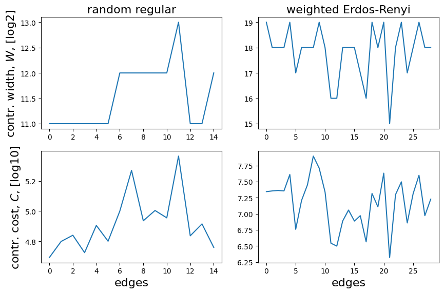
We detect that some of the trees in the second case reach a peak intermediate memory \(W \sim 19\), which corresponds to

\(2^{19}\mathrm{complex~numbers}\times 2\frac{\mathrm{real~numbers}}{\mathrm{complex~number}}\times 4\frac{\mathrm{bytes}}{\mathrm{single~precision~real~number}}=4\mathrm{~MB}\) (not big at all).

So what is hyperoptimization about? Finding the best contraction tree can depend on the underlying structure of the graph associated with the target contraction (here, the list of local expectation values in a QAOA Ansatz). Hyperoptimization leverages multiple path-finding methods and tunes their respective hyperparameters along the way to ensure that the resulting tree is truly optimal among all search strategies.

The aim of the hyperoptimization procedure is to minimize a cost function reflecting the overall cost of the contraction (minimize argument in the HyperOptimizer class), enabling us to target \(W\) (minimize=’size’), \(C\) (minimize=’flops’), the sum of all intermediate tensors written in memory (minimize=’write’) or a sum of the former and the later (minimize=f’combo-{alpha}’, with alpha being the prefactor of \(C\) in the cost function).

Finding the optimal contraction path in terms of speed and memory requirements is fundamental in many tasks. For our particular problem, this amounts to optimizing the execution of the cost function (the QAOA Ansatz energy), which enters another optimization loop in order to to solve the MaxCut instance.

9.3. Bayesian optimization loop

Once the contraction trajectories are pre-optimized, we can use some Bayesian optimizer to maximize the energy of the circuit with the QAOA Ansatz.

eps = 1e-6
bounds = [(0.0 + eps, qu.pi / 2 - eps)] * p + [(-qu.pi / 4 + eps, qu.pi / 4 - eps)] * p

We can monitor three times:

(1) the time of sampling the Bayesian surrogate to decide the next points where to evaluate the function (ask)

(2) the execution time for computing the cost function

(3) the time required to re-fit the surrogate after new information is fed into it (tell)

ask_time, cost_time, tell_time = [], [], []

batch_size = 10  # number of energy points per batch given to update the surrogate
num_iter = 20  # number of batches
ask_time, tell_time, cost_time, study = study_optimization_time_costs(
    terms_reg, opt_eco_reg, bounds, batch_size=batch_size, num_iter=num_iter
)

[I 2026-04-03 03:48:17,870] A new study created in memory with name: no-name-7f42b488-75b6-42ad-84f2-d13947ffda9d

After performing the optimization, we can break down the time cost of it:

fevals = [float(trial.value) for trial in study.trials]

fig, ax = plt.subplots(nrows=1, ncols=2, figsize=(10, 5 / 1.61))

ax[0].set_title("optimization times [seconds]", color="k")
ax[0].set_xlabel("batch number", color="k", size=10)
ax[1].set_title("cost function evaluations across all batches", color="k")
ax[1].set_xlabel("evaluation number", color="k", size=10)
ax[0].plot(ask_time, lw=2, label="ask=fit model")
ax[0].plot(tell_time, lw=2, label="tell=sample model")
ax[0].plot(cost_time, lw=2, label="avg. contr. per batch")
ax[0].legend()
ax[1].plot(fevals, lw=1);

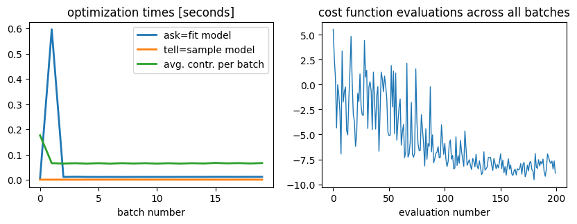
On the left hand plot we present the costs of asking, telling and contracting (average time cost per local expectation value among all the terms in the Hamiltonian). On the right plot we see the values of the cost function generated during the optimization procedure. The regressions observed in the value at later evaluations are due to exploration of points far from local minima, indicated on the Bayesian optimizer.

We observe an almost constant cost on the contraction times (as expected, since between calls of the Bayesian optimizer the execution caches the contraction paths and reexecutes them with new entries of the circuit tensors).

Since the example graphs above are small, we can solve the problem exactly, and directly evaluate the approximation ratio to the true answer:

max_energy, _ = brute_force_maxcut(nx.to_numpy_array(G_reg), terms_reg)
print(f"Approximation ratio: {100 * np.abs(min(fevals) / max_energy):.2f}%")

Approximation ratio: 74.58%

We can implement the same pipeline for the Erdos-Renyi graph. To do so, we wrapped up the loops of the last cells in the function study_optimization_time_costs, which can be found on src/qpe_toolbox/circuit/qaoa.py .

In this optimization procedure, the graph instances where so small that contraction costs have not been prohibitive for the optimization, so tuning the options of the HyperOptimizer was pointless. Nevertheless, if we scale up the instances or change the underlying couplings, it does become a requirement. The trees present on the former examples required \(C \simeq\) 4 and 7.5 on average for the random regular and Erdos-Renyi respectively, ultimately translating into average contraction times of around 2 seconds; for an increasing number of nodes and depth of the circuit, this will definetly rise if a proper path is not found.