4. Trotter-Suzuki decomposition of \(U(t)\)

In this notebook we introduce the Trotter-Suzuki decomposition to approximate the time-evolution operator \(U(t) = \exp(-i H t)\) for a Hamiltonian \(H\). We study the error and cost of the approximation. We take the nearest-neighbor 1D Heisenberg Hamiltonian to illustrate the method. We consider first and second order Trotter-Suzuki formulas.

4.1. Introduction

We start by introducing the general idea of Trotterization. We would like to compute the exponentiation of an operator \(H\). For small systems, it can be performed exactly by \(\texttt{quimb}\) or \(\texttt{scipy}\) linear algebra methods. In the \(\texttt{qpe-toolbox}\), the method get_U_exact of the Hamiltonian class returns the quantum gate implementing the exact time evolution using \(\texttt{quimb}\)’s expm matrix exponentiation routine. For larger systems however, computing the exact exponential is too expensive and we need to use approximations such as Trotterization.

Let us decompose the operator as \(H = A + B\). In practice, we decompose the Hamiltonian into a sum of operators whose exponentiation can be easily implemented, e.g. Pauli strings. When \(A\) and \(B\) commute, as for scalar numbers, the exponential of the sum is the product of exponentials:

\[ e^{A+B} = e^A e^B, \]

but in general \(A\) and \(B\) do not commute, hence the previous expression does not hold. Trotterization provides an approximation of the exponential of a sum based on the Baker-Campbell-Hausdorff formula.

The Trotter product formula gives the following expression:

\[ e^{A+B} = \lim_{r \to \infty} \left( e^{\frac{A}{r}} e^{\frac{B}{r}} \right)^r. \]

import time

import matplotlib.pyplot as plt
import numpy as np
import quimb as qu
import quimb.tensor as qtn
from tqdm import notebook as tqdm

from qpe_toolbox.hamiltonian import heisenberg_hamiltonian

plt.rcParams.update({"font.size": 12})

Now consider a general Hamiltonian, written as a sum of generally non-commuting terms:

\[ H = \sum_{\ell=1}^L H_\ell. \]

In this example, we take a 1D Heisenberg Hamiltonian with \(n=4\) spins and open boundary conditions. We want to compute the time-evolution operator \(U(t) = \exp(-iHt)\). Let us split the time interval into \(r\) timesteps of size \(t/r\).

n_qubits = 4
h_spin = heisenberg_hamiltonian(n_qubits)
qubit_reg = list(range(n_qubits))

4.1.1. First-order Trotter-Suzuki formula

The Trotter-Suzuki decompositions give approximations of \(U\) with increasing precision. The first-order Trotter-Suzuki decomposition is given by:

\[ e^{-i H \frac{t}{r}} = e^{-i H_1 \frac{t}{r}} \dots e^{-i H_L \frac{t}{r}} + \mathcal{O} \left(\left(\frac{t}{r}\right)^2 \right). \]

Along the full time evolution \(t\) errors accumulate:

\[ e^{-i H t} = \left( e^{-i H_1 \frac{t}{r}} \dots e^{-iH_L \frac{t}{r}} \right)^r + \mathcal{O} \left(\frac{t^2}{r}\right), \]

so that the error is linear in the timestep \(\delta t \equiv t/r\).

4.1.2. Second-order Trotter-Suzuki formula

Higher order decompositions can be obtained recursively. Here we go up to the second order Trotter-Suzuki decomposition:

\[ e^{-i H \frac{t}{r}} = e^{-i H_1 \frac{t}{2r}} \dots e^{-i H_{L-1} \frac{t}{2r}} e^{-i H_L \frac{t}{r}} e^{-i H_{L-1} \frac{t}{2r}} \dots e^{-i H_1 \frac{t}{2r}} + \mathcal{O} \left(\left(\frac{t}{r}\right)^3 \right), \]

which gives:

\[ e^{-i H t} = \left( e^{-i H_1 \frac{t}{2r}} \dots e^{-i H_{L-1} \frac{t}{2r}} e^{-i H_L \frac{t}{r}} e^{-i H_{L-1} \frac{t}{2r}} \dots e^{-i H_1 \frac{t}{2r}} \right)^r + \mathcal{O} \left(\frac{t^3}{r^2} \right). \]

The error is now quadratic in \(\delta t\).

In \(\texttt{qpe-toolbox}\), first- and second-order Trotterization are implemented by the get_trotter_step method of the Hamiltonian class.

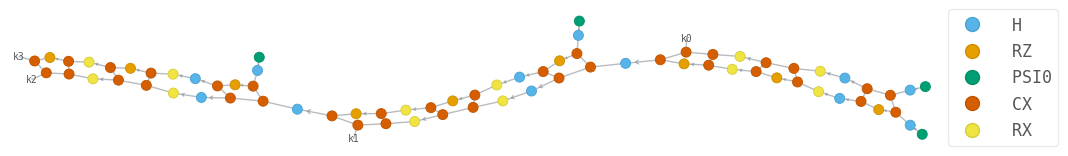
Below, we visualize the circuits for one timestep:

# First-order Trotter
dt = 1
trotter_routine = h_spin.get_trotter_step(dt, qubit_reg, trotter_order=1)

circ = qtn.Circuit(n_qubits)
circ.apply_gates(trotter_routine)
circ.draw(figsize=(14, 14))
circ.psi.draw(figsize=(12, 12), color={"PSI0", "H", "RX", "RZ", "CX"})

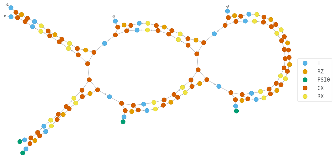
# Second-order Trotter
trotter_routine = h_spin.get_trotter_step(dt, qubit_reg, trotter_order=2)

circ = qtn.Circuit(n_qubits)
circ.apply_gates(trotter_routine)
circ.draw(figsize=(14, 14))
circ.psi.draw(figsize=(12, 12), color={"PSI0", "H", "RX", "RZ", "CX"})

4.2. Trotter error: full unitary distance as metric

Let us first use the distance of the full time evolution as a metric: \(||U_{\rm Trotter}^{\dagger}(t_f) U_{\rm exact}(t_f) - \mathbb{1}~||\)

We define a function that collects the errors defined for given times \(t\) in t_list, number of timesteps \(n_{steps}\) in ns_list and Trotterization order order.

NB: in this example we consider the Frobenius norm to define the error. Any other norm supported by quimb.norm can be used via the optional parameter ntype.

def errors_trotter_slice(t_list, ns_list, trotter_order, ntype="fro"):
    res = {"t": t_list, "n_s": ns_list, "errors_lists": [], "durations_lists": []}

    hamilt_matrix = h_spin.to_dense()
    id2n = qu.eye(2**n_qubits)

    for t in tqdm.tqdm(t_list):
        U_matrix = qu.expm(-1j * hamilt_matrix * t)

        errors = []
        durations = []
        for n_steps in tqdm.tqdm(ns_list, leave=False):
            st = time.time()
            circ = qtn.Circuit(n_qubits)
            dt = t / n_steps
            trotter_slice = h_spin.get_trotter_step(dt, qubit_reg, trotter_order)
            for _ in range(n_steps):
                circ.apply_gates(trotter_slice)
            U_trotter = circ.get_uni().to_dense()

            errors.append(qu.norm(U_matrix.H @ U_trotter - id2n, ntype=ntype))
            durations.append(time.time() - st)

        res["errors_lists"].append(errors)
        res["durations_lists"].append(durations)

    return res

We consider a sequence of evolution time growing like powers of \(2\) as in QPE: \(t_f = 2^kt, k = 1 \dots 6,\) where \(t\) is picked randomly in \([0,2\pi]\). We vary the number of Trotter steps between \(5\) and \(200\).

4.2.1. First order Trotter

Let us start with first order Trotter. The following cell should take a minute to run:

rng = np.random.default_rng(seed=42)
t_list = np.array([2 * np.pi * rng.random() * 2**j for j in range(6)])
ns_list = np.array([5, 10, 50, 100, 200])

res = errors_trotter_slice(t_list, ns_list, trotter_order=1)

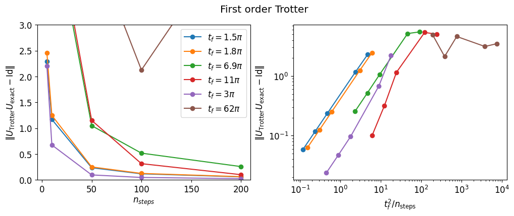
As seen in the introduction, we expect the error to scale like \(t_f^2 / n_{\rm steps}\). Let us plot the errors versus \(n_{\rm steps}\) (left, linear scale) and versus \(t_f^2 / n_{\rm steps}\) (right, log scale):

fig, (axl, axr) = plt.subplots(ncols=2, figsize=(12, 4))
for i, t in enumerate(res["t"]):
    axl.plot(
        res["n_s"], res["errors_lists"][i], "-o", label=rf"$t_f=${t / np.pi:.2g}$\pi$"
    )
    axr.loglog(t**2 / res["n_s"], res["errors_lists"][i], "-o")

axl.set_ylim(0, 3)
axl.legend()
axl.set_xlabel("$n_{steps}$")
axr.set_xlabel(r"${t_f^2}/{n_{\text{steps}}}$")
axl.set_ylabel(r"$\| U_{\mathrm{Trotter}}U_{\mathrm{exact}} - \mathrm{Id} \|$")
axr.set_ylabel(r"$\| U_{\mathrm{Trotter}}U_{\mathrm{exact}} - \mathrm{Id} \|$")
fig.suptitle("First order Trotter");

4.2.2. Second order Trotter

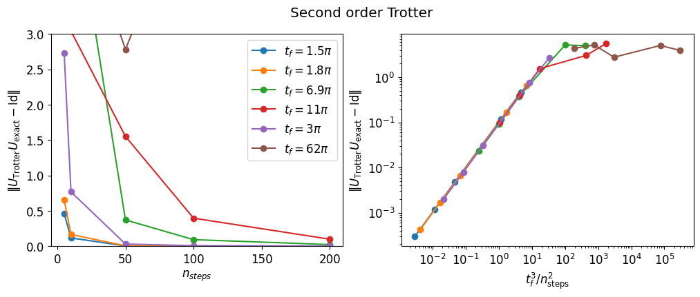
Similarly, we plot the errors reached with a second order Trotter formula, as a function of \(n_{\rm steps}\) (left, linear scale) and as a function of \(t_f^3 / n_{\rm steps}^2\) (right, log scale).

res2 = errors_trotter_slice(t_list, ns_list, trotter_order=2)

fig, (axl, axr) = plt.subplots(ncols=2, figsize=(12, 4))
for i, t in enumerate(res2["t"]):
    axl.plot(
        res2["n_s"], res2["errors_lists"][i], "-o", label=rf"$t_f=${t / np.pi:.2g}$\pi$"
    )
    axr.loglog(t**3 / res2["n_s"] ** 2, res2["errors_lists"][i], "-o")

axl.set_ylim(0, 3)
axl.legend()
axl.set_xlabel("$n_{steps}$")
axr.set_xlabel(r"${t_f^3}/n_{\text{steps}}^2$")
axl.set_ylabel(r"$\| U_{\mathrm{Trotter}}U_{\mathrm{exact}} - \mathrm{Id} \|$")
axr.set_ylabel(r"$\| U_{\mathrm{Trotter}}U_{\mathrm{exact}} - \mathrm{Id} \|$")

fig.suptitle("Second order Trotter");

4.2.3. Number of steps required to get below a given error

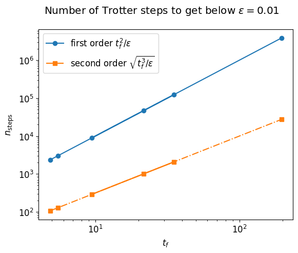
For the first order Trotter formula, since the error scales like \(t_f^2 / n_{\rm steps}\), to reach an error \(\epsilon\) requires a minimal number of steps:

\[ n_{\rm steps} = \mathcal{O} (t_f^2 / \epsilon) \]

Since in QPE maximum evolution time is \(t_f = \mathcal{O} (2^m)\) where \(m\) is number of phase bits, we get

\[ n_{\rm steps} = \mathcal{O} (2^{2m} / \epsilon). \]

As shown on the plot below, the number of Trotter steps quickly grows to about \(10^6\), which translates into at least as many CNOT gates. This is why in practice we use the second-order Trotter decomposition.

Trotter error at second order is \(\mathcal{O}(t_f^3 / n_{\rm steps}^2)\). Thus to reach an error \(\epsilon\) requires a number of steps scaling like

\[ n_{\rm steps} = \mathcal{O} (\sqrt{t_f^3 / \epsilon}) \]

Since in QPE the maximum evolution time is \(t_f = \mathcal{O} (2^m)\) where \(m\) is number of phase bits, we get

\[ n_{\rm steps} = \mathcal{O} (\sqrt{2^{3m} / \epsilon}) \]

epsilon = 1e-2

fig, ax = plt.subplots()
ax.loglog(t_list, t_list**2 / epsilon, "-o", label=r"first order $t_f^2/\epsilon$")
ax.loglog(
    t_list,
    np.sqrt(t_list**3 / epsilon),
    "-.s",
    label=r"second order $\sqrt{t_f^{3}/\epsilon}$",
)
ax.set_xlabel(r"$t_f$")
ax.set_ylabel(r"$n_{\text{steps}}$")
ax.legend()
fig.suptitle(f"Number of Trotter steps to get below $\\epsilon = {epsilon}$");

4.2.4. Number of CNOT gates required to get below a given error

Here we investigate the number of entangling gates required to run a Trotter time evolution within a given error bound \(\varepsilon\).

The Trotter decomposition expresses the evolution operator as a product of exponential of Pauli strings. Let us describe the algorithm for the exponentiation of Pauli strings.

4.2.4.1. Quantum circuit for exponentiation of Pauli strings

The different terms in the Hamiltonian can be written as Pauli strings, i.e. using the Pauli operator basis:

\[ H_\ell = U_1 \otimes U_2 \otimes \dots \otimes U_n, \qquad U_k \in \{\mathbb{1}, X, Y, Z\}, \]

where \(n\) is the number of qubits required to represent the Hilbert space.

Here we present the algorithm to exponentiate \(H_\ell\), i.e. to encode \( e^{-i H_\ell t} = e^{ -i t U_1 \otimes U_2 \otimes \dots \otimes U_n }. \) A mathematical demonstration of a similar algorithm can be found in Fleury, Lacomme, Quantum circuit for exponentiation of Hamiltonians: an algorithmic description based on tensor products, arXiv:2501.17780.

Let us first state the following two properties :

• \( e^{-i t Z} = R_Z(2t) \) by definition.

• \( e^{-i t Z_{i_1} Z_{i_2} \dots Z_{i_M}} = CX_{i_1 i_2} CX_{i_2 i_3} \dots CX_{i_{M-1} i_M} \left( \mathbb{1}^{\otimes (i_M-1)} \otimes R_Z(2t) \otimes \mathbb{1}^{\otimes (n - i_M - 1)} \right) CX_{i_{M-1} i_M} CX_{i_{M-1} i_{M-2}} \dots CX_{i_1 i_2} \) (see arXiv:2501.17780).

The algorithm proceeds as follows:

1. First, apply basis rotations to bring all qubits into the \(Z\) basis:

   • if \(U_k=X\), apply a Hadamard gate \(H\) to the \(k\)-th qubit.

   • if \(U_k=Y\), apply a rotation gate \(R_X(\pi/2)\) to the \(k\)-th qubit.

2. Then, apply a sequence of CNOT gates between \(i_k\) and \(i_{k+1}\) where \(i_k\) are the indices of non-identity operators in the strings.

3. Apply \(R_Z(2t)\) to the last qubit on which a non-identity Pauli operator is acting.

4. Apply the reversed CNOT sequence.

5. Bring the qubits back to their original basis applying the inverse rotations.

This algorithm is executed by the rotation_gates function from \(\texttt{qpe-toolbox}\) ‘s hamiltonian module.

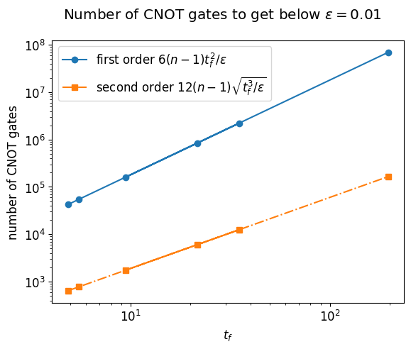
4.2.4.2. CNOT gate count

Thus, the algorithm to implement a Pauli string exponential \(\exp( i \theta P_1 ... P_K )\), where \(P_i \in \{X,Y,Z\}\) are Pauli operators distinct from Identity, uses \(2 (K - 1)\) CNOT gates, where \(K\) is the length of the Pauli string.

For the Heisenberg Hamiltonian:

\[ H = \frac{J}{2} \sum_{i=0}^{n-2} \left( X_i X_{i+1} + Y_i Y_{i+1} + Z_i Z_{i+1} \right). \]

• One Trotter slice (first order):

\[ e^{ - i H dt } = \prod_{i=0}^{n-2} e^{-i X_i X_{i+1} dt J/2} e^{-i Y_i Y_{i+1} dt J/2} e^{-i Z_i Z_{i+1} dt J/2} + \mathcal{O} (dt^2) \]

is thus implemented with \(6(n-1)\) CNOT gates (3 axis, for each axis a length-2 Pauli string).

This gives a total CNOT gate count for the Trotterization of \(U(t)\):

\[ 6(n - 1)n_{steps} \qquad \mathrm{CNOT~gates}\]

• Second order:

\[ e^{ - i H dt } = \prod_{j=0}^{n-2} e^{-i X_j X_{j+1} dt J/4} e^{-i Y_j Y_{j+1} dt J/4} e^{-i Z_j Z_{j+1} dt J/4} \prod_{k=0}^{n-2} e^{-i Z_{n-2-k} Z_{n-1-k} dt J/4} e^{-i Y_{n-2-k} Y_{n-1-k} dt J/4} e^{-i X_{n-2-k} X_{n-1-k} dt J/4} + \mathcal{O} (dt^3). \]

Total CNOT gate count second order Trotterization:

\[ 12(n - 1)n_{steps} \qquad \mathrm{CNOT~gates}.\]

Note that the two neighboring \(e^{-i Z_{n-2} Z_{n-1} dt J/4}\) terms could be merged, as well as the \(e^{-i X_0 X_1 dt J/4}\) terms from neighboring Trotter steps, to reduce the total CNOT gate count. Here we only implement the most naive version of second-order Trotterization: in general, one should merge the two occurences of the last Hamiltonian term.

fig, ax = plt.subplots()
ax.loglog(
    t_list,
    6 * (n_qubits - 1) * t_list**2 / epsilon,
    "-o",
    label=r"first order $6(n-1)t_f^2/\epsilon$",
)
ax.loglog(
    t_list,
    np.sqrt(12 * (n_qubits - 1) * t_list**3 / epsilon),
    "-.s",
    label=r"second order $12(n-1)\sqrt{t_f^{3}/\epsilon}$",
)
ax.set_xlabel(r"$t_f$")
ax.set_ylabel(r"number of CNOT gates")
ax.legend()
fig.suptitle(f"Number of CNOT gates to get below $\\epsilon = {epsilon}$")

Text(0.5, 0.98, 'Number of CNOT gates to get below $\\epsilon = 0.01$')

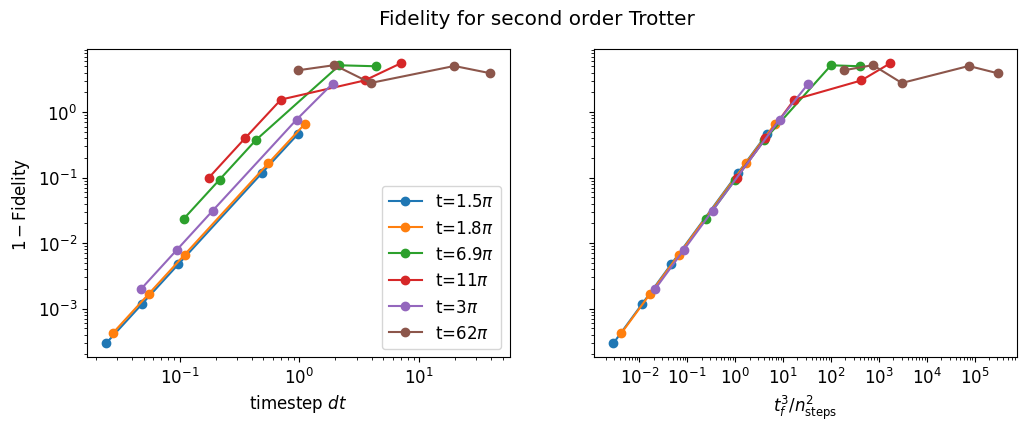
4.3. Fidelity as an error metric

In a QPE experiment, we are interested in the time evolution of an Hamiltonian eigenstate. Let us therefore consider the quantum fidelity as an error metric. Quantum fidelity is defined as \(|\langle\psi_{\rm exact}(t) | \psi_{\rm trotter}(t)\rangle|^2\). We consider second order Trotter decomposition

def fidelities_trotter_slice(n_qubits, t_list, ns_list, trotter_order):
    res = {"t": t_list, "n_s": ns_list, "errors_lists": [], "durations_lists": []}

    reg = list(range(n_qubits))
    h_spin = heisenberg_hamiltonian(n_qubits)
    hamilt_matrix = h_spin.to_dense()
    _eigvals, eigvecs = np.linalg.eigh(hamilt_matrix)

    psi0 = eigvecs[:, 0]
    psi0_mps = qtn.MatrixProductState.from_dense(psi0)

    for t in tqdm.tqdm(t_list):
        U = qu.expm(-1j * hamilt_matrix * t)
        psi_ref = U @ psi0

        errors = []
        durations = []
        for n_steps in tqdm.tqdm(ns_list, leave=False):
            st = time.time()
            circ = qtn.Circuit(n_qubits, psi0=psi0_mps)
            dt = t / n_steps
            trotter_slice = h_spin.get_trotter_step(dt, reg, trotter_order)
            for _ in range(n_steps):
                circ.apply_gates(trotter_slice)

            errors.append(
                abs(1 - qu.fidelity(circ.psi.to_dense(), psi_ref, squared=True))
            )
            durations.append(time.time() - st)

        res["errors_lists"].append(errors)
        res["durations_lists"].append(durations)
    return res

res2f = fidelities_trotter_slice(n_qubits, t_list, ns_list, trotter_order=2)

fig, (axl, axr) = plt.subplots(ncols=2, figsize=(12, 4), sharey=True)
for i, t in enumerate(res2["t"]):
    axl.loglog(
        t / res2["n_s"], res2["errors_lists"][i], "-o", label=rf"t={t / np.pi:.2g}$\pi$"
    )
    axr.loglog(t**3 / res2["n_s"] ** 2, res2["errors_lists"][i], "-o")

axl.legend()
axl.set_xlabel("timestep $dt$")
axl.set_ylabel(r"$1-\text{Fidelity}$")
axr.set_xlabel(r"${t_f^3}/n_{\text{steps}}^2$")
fig.suptitle("Fidelity for second order Trotter");

This ends our simple introduction on Trotter-Suzuki decomposition. For the reader interested in going further, we refer to this paper by Andrew M. Childs that gives a theoretical study of Trotter error with a focus on Hamiltonian simulation.