10. Variational circuit preparation I
In this tutorial, we demonstrate two complementary classical pre-processing techniques to prepare a quantum circuit that approximates the ground state of a given Hamiltonian. Such a circuit can be used as an initial state in quantum phase estimation (QPE) or other quantum algorithms.
We consider the 1D transverse-field Ising model and build a brick-wall circuit of general two-qubit gates, where each of them can be parametrized by at most 3 CNOT gates and 15 elementary one-qubit gates (for more details, read Vatan and Williams, Phys. Rev. A 69, 032315 (2004)).
The two approaches are:
Global optimization - all parameters of the circuit are optimized simultaneously using gradient-based methods (L-BFGS) via auto-differentiation. The parameters are the 15 real entries of the SU(4) gates, and the unitarity is enforced by construction.
Local optimization - the circuit is represented as a tensor network, and the individual tensor entries are optimized locally. The optimization is performed by sweeping through the tensors, similar to DMRG, and often yields high-fidelity states.
We compare the performance of both strategies and also illustrate a sequential depth optimisation that starts from a shallow circuit and progressively increases the depth, reusing parameters from shallower layers.
The target state is obtained by DMRG (via quimb.tensor.DMRG2), which provides a reference energy and the numerically exact ground state.
import os

os.environ["OPENBLAS_NUM_THREADS"] = "1"
os.environ["NUMBA_NUM_THREADS"] = "1"
os.environ["OMP_NUM_THREADS"] = "1"
os.environ["MKL_NUM_THREADS"] = "1"
os.environ["JAX_ENABLE_X64"] = "True"

import autoray
import matplotlib.pyplot as plt
import numpy as np
import quimb.tensor as qtn

# Local imports from qpe_toolbox
from qpe_toolbox.circuit import ansatz_circuit_su4, su4swap_gate_param_gen, tn_fit
from qpe_toolbox.hamiltonian import Hamiltonian
10.1. Hamiltonian: 1D Transverse-Field Ising (TFI) model
We consider a chain of \(n\) spins with open boundaries. The Hamiltonian reads
with \(g_x = -1.1\) and \(g_{zz} = -1.0\). We take \(n = 8\) sites.
First, we compute the ground state using DMRG (via qtn.DMRG2). This gives us the target state GS and the exact energy.
# --- Hamiltonian definition ---
n_qubits = 8
gx, gzz = -1.1, -1.0
terms = []
for x in range(n_qubits):
    terms.append((gx, "x", [x]))  # transverse field
for x in range(n_qubits - 1):
    terms.append((gzz, "zz", [x, x + 1]))  # nearest-neighbour coupling
ham = Hamiltonian(terms, n_qubits)
mpo = ham.to_mpo()

# --- DMRG reference ground state ---
dmrg = qtn.DMRG2(mpo)
dmrg.solve(max_sweeps=16, tol=1e-8, bond_dims=64, verbosity=0)
GS = dmrg.state
dmrg_energy = np.real(dmrg.energy)
print(f"*** DMRG reference energy: {dmrg_energy:12.10f}")
print()
*** DMRG reference energy: -10.4564576523
10.2. Global Optimization
The circuit is built from SU(4) gates, each parameterized by 15 real numbers. We define a loss function that computes the expectation value of the Hamiltonian MPO with respect to the state produced by the circuit. The gradient is obtained via automatic differentiation (JAX). Ref: Haghshenas et al. Phys. Rev. X 12, 011047 (2022), Tensor Network Training of Quantum Circuits
Three global optimization strategies are compared:
Standard L-BFGS on a fixed-depth circuit.
Basin-hopping - a global optimisation method that helps escape local minima.
Sequential layer-wise optimization, where a shallower circuit is optimized first, and its parameters are used to initialize a deeper one.
def loss_circ(circ, mpo):
    """
    Loss function: expectation value of the MPO Hamiltonian with respect to
    the state produced by the circuit.
    """
    psi = circ.psi
    psiH = psi.H
    norm_tn = psiH & psi
    psi.align_(mpo, psiH)
    energy_tn = psiH & mpo & psi
    energy = autoray.do("real", energy_tn.contract())
    norm = autoray.do("real", norm_tn.contract())
    return (energy / norm).real


def make_circuit_optimizer(circ, mpo):
    """
    Factory to create a TNOptimizer for a circuit with the given MPO.

    Uses L-BFGS-B (or basin-hopping) and JAX for gradients.
    """
    return qtn.TNOptimizer(
        circ,
        loss_circ,
        loss_constants={"mpo": mpo},
        autodiff_backend="jax",
        optimizer="L-BFGS-B",
        progbar=False,
    )
10.2.1. 1. Direct L-BFGS optimization
print("*** Global L-BFGS optimization")
depth = 6
circ = ansatz_circuit_su4(n_qubits, depth)
circ_opt = make_circuit_optimizer(circ, mpo)
optimal_circ = circ_opt.optimize(n=10000, tol=1e-8)
ovlp = (dmrg.state.H & optimal_circ.psi).contract()
print(
    f" # parameters = {circ_opt.d: 4d}",
    f" Energy = {circ_opt.loss: >12.8f}",
    f" Error = {np.abs(1 - circ_opt.loss / dmrg_energy): >10.3e}",
    f" 1-F = {1 - np.abs(ovlp) ** 2: >10.3e}",
)
print()
*** Global L-BFGS optimization
# parameters = 630 Energy = -10.45638540 Error = 6.910e-06 1-F = 1.332e-05
10.2.2. 2. Basin-hopping optimization
Basin-hopping performs random steps in parameter space followed by a local minimization. Here we use 5000 iterations with 10 hops per step and a temperature of 0.1.
print("*** Global L-BFGS optimization + Basin-hopping ")
depth = 6
circ = ansatz_circuit_su4(n_qubits, depth)
circ_opt = make_circuit_optimizer(circ, mpo)
optimal_circ = circ_opt.optimize_basinhopping(n=5000, nhop=10, temperature=0.1)
ovlp = (dmrg.state.H & optimal_circ.psi).contract()
print(
    f" # parameters = {circ_opt.d: 4d}",
    f" Energy = {circ_opt.loss: >12.8f}",
    f" Error = {np.abs(1 - circ_opt.loss / dmrg_energy): >10.3e}",
    f" 1-F = {1 - np.abs(ovlp) ** 2: >10.3e}",
)
print()
*** Global L-BFGS optimization + Basin-hopping
# parameters = 630 Energy = -10.45638978 Error = 6.491e-06 1-F = 4.192e-06
10.2.3. 3. Sequential layer-wise optimization
We start from depth 1 and increase the depth one layer at a time, always reusing the parameters from the shallower circuit as initial guess.
print("*** Global L-BFGS sequential optimization ")
depths_global = []
errors_global = []
rng = np.random.default_rng(42)

circ = ansatz_circuit_su4(n_qubits, 1, rng=rng)
circ_opt = make_circuit_optimizer(circ, mpo)
optimal_circ = circ_opt.optimize(n=10000, tol=1e-8)
ovlp = (dmrg.state.H & optimal_circ.psi).contract()
err = np.abs(1 - circ_opt.loss / dmrg_energy)
depths_global.append(1)
errors_global.append(err)
print(
    f" # parameters = {circ_opt.d: 4d}",
    f" Energy = {circ_opt.loss: >12.8f}",
    f" Error = {err: >10.3e}",
    f" 1-F = {1 - np.abs(ovlp) ** 2: >10.3e}",
)

for ii in range(2, depth + 1):
    # grow the optimized circuit by one SU4SWAP layer initialized close to identity
    for start in range(2):
        for q in range(start, n_qubits - 1, 2):
            optimal_circ.apply_gate(
                "SU4SWAP",
                *(0.1 * rng.random(15)),
                q,
                q + 1,
                gate_round=ii - 1,
                parametrize=True,
            )
    circ_opt = make_circuit_optimizer(optimal_circ, mpo)
    optimal_circ = circ_opt.optimize(n=10000, tol=1e-8)
    ovlp = (dmrg.state.H & optimal_circ.psi).contract()
    err = np.abs(1 - circ_opt.loss / dmrg_energy)
    depths_global.append(ii)
    errors_global.append(err)
    print(
        f" # parameters = {circ_opt.d: 4d}",
        f" Energy = {circ_opt.loss: >12.8f}",
        f" Error = {err: >10.3e}",
        f" 1-F = {1 - np.abs(ovlp) ** 2: >10.3e}",
    )
print()
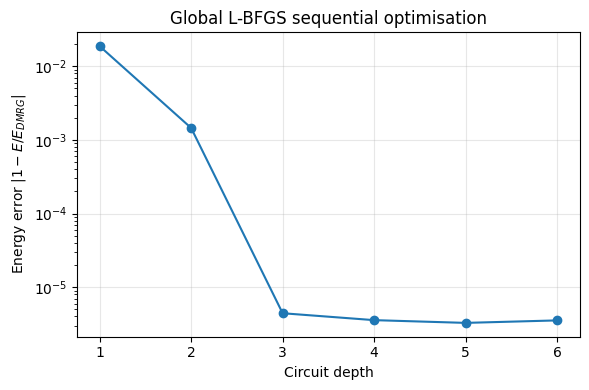
*** Global L-BFGS sequential optimization
# parameters = 105 Energy = -10.26060113 Error = 1.873e-02 1-F = 2.611e-01
# parameters = 210 Energy = -10.44128128 Error = 1.451e-03 1-F = 6.541e-03
# parameters = 315 Energy = -10.45641137 Error = 4.427e-06 1-F = 9.179e-06
# parameters = 420 Energy = -10.45642036 Error = 3.566e-06 1-F = 7.253e-06
# parameters = 525 Energy = -10.45642342 Error = 3.273e-06 1-F = 6.531e-06
# parameters = 630 Energy = -10.45642066 Error = 3.538e-06 1-F = 6.245e-06
10.2.3.1. Plot: Error vs depth for global sequential optimization
plt.figure(figsize=(6, 4))
plt.plot(depths_global, errors_global, marker="o", linestyle="-")
plt.xlabel("Circuit depth")
plt.ylabel("Energy error $|1 - E/E_{DMRG}|$")
plt.title("Global L-BFGS sequential optimisation")
plt.yscale("log")
plt.grid(visible=True, alpha=0.3)
plt.tight_layout()
plt.show()
10.3. Local Optimization
Ref: Causer et al. Phys. Rev. Research 6, 033062 (2024), Gibbs and Cincio, Quantum 9, 1789 (2025).
In this approach, the circuit is represented as a tensor network (each two-qubit gate is a 4-leg tensor). We optimize the tensor entries directly using a local (sweeping) optimization based on the polar decomoposition that maximize the fidelity.
We use the function tn_fit from qpe_toolbox.circuit, which performs a local optimisation of the tensor network.
We first optimise a fixed depth-6 circuit, and then demonstrate a sequential depth optimisation that starts from depth 1 and increases depth, reusing the tensor entries from the previous depth.
# --- Fixed depth 6 ---
print("*** Local optimization")
depth = 6
circ = ansatz_circuit_su4(
    n_qubits=n_qubits, depth=depth, param_scaling=1.0, parametrize=False
)

tn = circ.psi
tn_fit(tn, GS, tags="SU4SWAP", steps=100000, tol=1e-8)

ovlp = (dmrg.state.H & tn).contract()
tnH = tn.H
tn.align_(mpo, tnH)
energy_tn = tnH & mpo & tn
ene = autoray.do("real", energy_tn.contract(all))

print(
    f"Depth = {depth:2d}   Energy = {ene:12.8f}   Error = {np.abs(1 - ene / dmrg_energy):10.3e}   1-F = {1 - np.abs(ovlp) ** 2:10.3e}"
)
print()
*** Local optimization
Depth = 6 Energy = -10.45626977 Error = 1.797e-05 1-F = 1.794e-05
10.3.1. Sequential depth optimization (local)
Starting from a depth-1 circuit, we optimise it, then add a layer, reusing the tensor entries from the previous circuit as initialisation.
print("*** Local sequential optimization")
# --- Modified: store errors vs depth ---
depths_local = []
errors_local = []

circ = ansatz_circuit_su4(
    n_qubits=n_qubits, depth=1, param_scaling=1.0, parametrize=False
)

tn = circ.psi
tn_fit(tn, GS, tags="SU4SWAP", steps=10000, tol=1e-8)

ovlp = (dmrg.state.H & tn).contract()
tnH = tn.H
tn.align_(mpo, tnH)
energy_tn = tnH & mpo & tn
ene = autoray.do("real", energy_tn.contract(all))
err = np.abs(1 - ene / dmrg_energy)
depths_local.append(1)
errors_local.append(err)

print(
    f"Depth = {1:2d}   Energy = {ene:12.8f}   Error = {err:10.3e}   1-F = {1 - np.abs(ovlp) ** 2:10.3e}"
)

rng = np.random.default_rng(42)

for ii in range(2, depth + 1):
    # grow the optimized network by one brick-wall layer of SU4SWAP gates,
    # initialized close to the identity (small parameters)
    tags = ["SU4SWAP", f"ROUND_{ii - 1}"]
    for start in range(2):
        for q in range(start, n_qubits - 1, 2):
            gate = su4swap_gate_param_gen(1e-2 * rng.random(15))
            tn.gate_(gate, (q, q + 1), tags=tags, contract=False)

    tn_fit(tn, GS, tags="SU4SWAP", steps=10000, tol=1e-8)

    ovlp = (dmrg.state.H & tn).contract()
    tnH = tn.H
    tn.align_(mpo, tnH)
    energy_tn = tnH & mpo & tn
    ene = autoray.do("real", energy_tn.contract(all))
    err = np.abs(1 - ene / dmrg_energy)
    depths_local.append(ii)
    errors_local.append(err)

    print(
        f"Depth = {ii:2d}   Energy = {ene:12.8f}   Error = {err:10.3e}   1-F = {1 - np.abs(ovlp) ** 2:10.3e}"
    )
print()
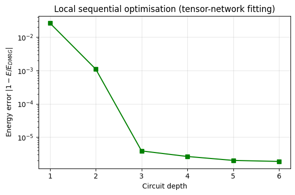
*** Local sequential optimization
Depth =  1   Energy = -10.18106100   Error =  2.634e-02   1-F =  8.268e-02
Depth = 2 Energy = -10.44499676 Error = 1.096e-03 1-F = 3.466e-03
Depth = 3 Energy = -10.45641720 Error = 3.868e-06 1-F = 6.445e-06
Depth = 4 Energy = -10.45643009 Error = 2.636e-06 1-F = 4.525e-06
Depth = 5 Energy = -10.45643662 Error = 2.011e-06 1-F = 3.416e-06
Depth = 6 Energy = -10.45643808 Error = 1.872e-06 1-F = 3.065e-06
10.3.1.1. Plot: Error vs depth for local sequential optimization
plt.figure(figsize=(6, 4))
plt.plot(depths_local, errors_local, marker="s", linestyle="-", color="green")
plt.xlabel("Circuit depth")
plt.ylabel("Energy error $|1 - E/E_{DMRG}|$")
plt.title("Local sequential optimisation (tensor-network fitting)")
plt.yscale("log")
plt.grid(visible=True, alpha=0.3)
plt.tight_layout()
plt.show()
10.4. Discussion
The results above show that:
Global optimisation with L-BFGS can already find a good approximation, but basin-hopping and sequential layer-wise initialization often improve the fidelity and energy.
Local optimisation (tensor-network fitting) yields very high fidelity (low infidelity) and energies very close to the DMRG reference. The sequential depth variant further improves convergence.
Both approaches provide a classical pre-processing step to generate a high-quality initial state for quantum algorithms such as QPE. The choice between them depends on the available infrastructure (automatic differentiation, global vs local optimizers) and the desired accuracy