11. Variational Circuit Preparation II
This script implements a local optimization to prepare a quantum circuit that approximates the ground state of a given Hamiltonian. Unlike the straightforward global fitting of the entire circuit (as in circuit_preparation_opt.py), this version performs a sweeping algorithm that optimizes the circuit layer by layer, sweeping from the bottom (first layer) to the top (last layer) and back.
The method is useful when the circuit is deep. By sequentially updating each layer while approximating the rest of the circuit with finite bond dimensions MPSs, we can efficiently achieve high fidelity with the target MPS.
Ref: Gibbs and Cincio, Quantum 9, 1789 (2025).
We demonstrate the technique on the 1D transverse-field Ising model, using a brick-wall SU(4) circuit. The target state is obtained via DMRG. The algorithm constructs the circuit’s MPS layer by layer, and at each step it uses the tensor-network fitting routine to update the tensors of a given layer so that the overlap with the target state is maximized.
The main steps are:
Define the Hamiltonian and compute its ground state
GSvia DMRG.Build an initial random SU(4) brick-wall circuit of a given depth.
Perform an initial sweep (down then up) that optimizes the parameters layer by layer, reusing the partially optimized MPS from previous layers.
After each full sweep, compute the energy and fidelity of the current circuit against the DMRG target.
Repeat for a number of sweeps (1000 in this example) to converge.
This approach is inspired by the local optimization idea but applies it in a sequential, sweep-based fashion, which often leads to faster convergence for deep circuits.
import os

# Limit threading for reproducibility and performance.
os.environ["NUMBA_NUM_THREADS"] = "1"
os.environ["OMP_NUM_THREADS"] = "1"
os.environ["MKL_NUM_THREADS"] = "1"

import autoray
import matplotlib.pyplot as plt
import numpy as np
import quimb.tensor as qtn
from quimb.tensor import DMRG2

from qpe_toolbox.circuit import ansatz_circuit_su4, tn_fit
from qpe_toolbox.hamiltonian import Hamiltonian
11.1. Script Execution: Layer-by-Layer Sweep
We now apply the tensor-network fitting in a sweeping fashion:
We start from an initial product state
psi0 = |0...0>.We build the circuit layer by layer. The ansatz consists of SU(4) gates arranged in a brick-wall pattern. Each layer is a collection of two-qubit gates that act on disjoint pairs.
We maintain two lists of MPS:
mpsK(the “forward” state, built from the bottom) andmpsB(the “backward” state, built from the top). The goal is to make the overlap<mpsB|circuit|mpsK>as close to 1 as possible, wherecircuitis the full unitary.In the sweep-down phase, we start from the top layer and work downwards. For each layer, we:
Form a trial circuit consisting of the current
mpsK(which already contains all layers below this one) plus the gates of the current layer.Fit the tensors of that layer so that the resulting MPS matches the current
mpsB(which contains all layers above this one, already optimized).After updating the layer, we update
mpsBby applying the conjugated gates (using MPO) to move one layer down.
In the sweep-up phase, we reverse the direction: we start from the bottom and work upwards, updating each layer similarly.
After each full sweep (down+up), we evaluate the energy and fidelity of the full circuit against the DMRG target.
This approach is very similar to the DMRG sweep algorithm, but with the roles of the Hamiltonian and the unitary gates interchanged. It allows us to efficiently optimize deep circuits while keeping bond dimensions manageable.
We run 1000 sweeps; the algorithm should converge to a state that closely approximates the ground state.
11.1.1. 1. Hamiltonian and DMRG Reference
We set up the 1D transverse-field Ising model:
with \(g_x = -1.1\) and \(g_{zz} = -1.0\). We take 8 qubits. The ground state is computed with DMRG (bond dimension 64, 16 sweeps) and used as the target.
## hamiltonian
n_qubits = 4
list_paulis = ["I", "X", "Y", "Z"]
gx, gzz = -1.1, -1.0
terms = []
for x in range(n_qubits):
    terms.append((gx, "x", [x]))
for x in range(n_qubits - 1):
    terms.append((gzz, "zz", [x, x + 1]))
ham = Hamiltonian(terms, n_qubits)
mpo = ham.to_mpo()

# Run DMRG to get the target state and energy.
dmrg = DMRG2(mpo)
dmrg.solve(max_sweeps=16, tol=1e-8, bond_dims=64, verbosity=0)
GS = dmrg.state
dmrg_energy = np.real(dmrg.energy)
print("*** DMRG reference energy:", dmrg_energy)
print()
*** DMRG reference energy: -5.089485813291186
11.1.2. 2. Circuit Initialization and Layer Preparation
We build an ansatz circuit of a given depth (here 6). The circuit is a brick-wall of SU(4) gates.
We also build an initial product state psi0 = |0...0>.
Then we create two lists:
mpsK: starts withpsi0. For each layer (from bottom to top), we apply the corresponding gates as MPOs to build the forward MPS.mpsB: starts with the conjugate of the target stateGS.H. This will be updated as we sweep from the top downwards.
These lists are used in the sweeping algorithm to keep track of the partially contracted states.
## initialise
depth = 6
psi0 = qtn.MPS_computational_state("0" * n_qubits)
circ = ansatz_circuit_su4(
    n_qubits=n_qubits, depth=depth, param_scaling=0.1, parametrize=False, psi0=psi0
)
circ_P = circ.psi
circ_G = list(circ.gates)

# Build the forward MPS for each layer (from bottom to top).
mpsB = []
mpsB.append(GS.H)
mpsK = []
mpsK.append(psi0)
for ii in range(depth - 1):
    # Get gates belonging to this round (layer).
    mpos = [gate.build_mpo(L=n_qubits) for gate in circ_G if gate.round == ii]
    tmp = mpsK[-1]
    for jj in mpos:
        tmp = tmp.gate_with_submpo(jj, transpose=False, max_bond=32, cutoff=1e-10)
    mpsK.append(tmp)
11.1.3. 3. Sweeping Optimization
We perform a number of full sweeps (sweep from 0 to 499). Each sweep consists of two phases:
Sweep down: from the top layer (
depth-1) down to layer 0.For a given layer
ii(top to bottom), we construct a trial circuittrialfrommpsK[-1](which contains all layers below) and the gates of that layer.We call
tn_fitto optimize the tensors of that layer, selected by their layer tagROUND_{depth-1-ii}, so that the trial MPS matches the currentmpsB[-1](which contains all layers above, already optimized).We then copy the optimized tensor data back into the main circuit representation (
circ_Pandcirc_G).We update
mpsBby applying the conjugated gates (as MPOs) to move the boundary one layer down.
Sweep up: from the bottom layer (0) up to
depth-1.Similar to sweep down, but we start from
mpsK[-1]and update layers from bottom to top.We also update
mpsKby applying the (non-conjugated) gates to move the forward boundary up.
After each full sweep, we contract the full circuit with the MPO to compute the energy and the overlap with the DMRG state. This gives a measure of convergence.
# Initialize lists to store convergence data
sweep_numbers = []
energy_errors = []
infidelities = []
energies = []

# Print a header for the convergence output
print("Sweep    Energy         Error       1-Fidelity")
print("------------------------------------------------")

ene_old = float("nan")
ene = float("nan")

n_sweeps = 1000
for sweep in range(n_sweeps):
    ## Sweep down: optimize layers from top to bottom.
    for ii in range(depth - 1):
        # Build trial circuit from current mpsK (layers below) + gates of this layer.
        trial = qtn.Circuit(psi0=mpsK.pop())
        gates = [gate for gate in circ_G if gate.round == depth - 1 - ii]
        for gate in gates:
            trial.apply_gate(gate)

        tn = trial.psi
        # Fit the SU4SWAP tensors of this layer to match the current mpsB (layers above).
        tn_fit(
            tn,
            mpsB[-1].H,  # note: mpsB stores the conjugate, so we use its adjoint.
            tags=f"ROUND_{depth - 1 - ii}",
            steps=10,  # inner ALS sweeps per layer update
            tol=1e-12,
            contract_optimize="auto-hq",
            progbar=False,
        )

        # Copy the optimized tensor data back into the master circuit tensors.
        g0 = tn.select_tensors("ROUND_" + str(depth - 1 - ii), "any")
        g1 = circ_P.select_tensors("ROUND_" + str(depth - 1 - ii), "any")
        gate_indices = [
            i for i, gate in enumerate(circ_G) if gate.round == depth - 1 - ii
        ]
        for t0, t1, ig in zip(g0, g1, gate_indices, strict=True):
            t1.modify(data=t0.data)
            old = circ_G[ig]
            circ_G[ig] = qtn.circuit.Gate.from_raw(
                t0.data, qubits=old.qubits, controls=old.controls, round=old.round
            )

        # Update mpsB: apply the conjugated gates (as MPOs) to move down one layer.
        mpos = [circ_G[ig].build_mpo(L=n_qubits) for ig in gate_indices]
        mpos.reverse()  # reverse order because we are conjugating and moving down

        tmp = mpsB[-1]
        for jj in mpos:
            tmp = tmp.gate_with_submpo(jj, transpose=True, max_bond=32, cutoff=1e-12)
        mpsB.append(tmp)

    ## Sweep up: optimize layers from bottom to top.
    for ii in range(depth - 1):
        # Build trial circuit from current mpsK[-1] (which has all layers below) + gates of this layer.
        trial = qtn.Circuit(psi0=mpsK[-1])
        gates = [gate for gate in circ_G if gate.round == ii]
        for gate in gates:
            trial.apply_gate(gate)

        tn = trial.psi
        # Fit the SU4SWAP tensors of this layer to match the current mpsB (top part, already optimized).
        tn_fit(
            tn,
            mpsB.pop().H,  # use the top part; pop removes the last element (which corresponds to the layer just below)
            tags=f"ROUND_{ii}",
            steps=10,
            tol=1e-12,
            contract_optimize="auto-hq",
            progbar=False,
        )

        # Copy optimized data back to master circuit.
        g0 = tn.select_tensors("ROUND_" + str(ii), "any")
        g1 = circ_P.select_tensors("ROUND_" + str(ii), "any")
        gate_indices = [i for i, gate in enumerate(circ_G) if gate.round == ii]
        for t0, t1, ig in zip(g0, g1, gate_indices, strict=True):
            t1.modify(data=t0.data)
            old = circ_G[ig]
            circ_G[ig] = qtn.circuit.Gate.from_raw(
                t0.data, qubits=old.qubits, controls=old.controls, round=old.round
            )

        # Update mpsK: apply the (non-conjugated) gates to move the forward boundary up.
        mpos = [circ_G[ig].build_mpo(L=n_qubits) for ig in gate_indices]

        tmp = mpsK[-1]
        for jj in mpos:
            tmp = tmp.gate_with_submpo(jj, transpose=False, max_bond=32, cutoff=1e-12)
        mpsK.append(tmp)

    # ## 4. Evaluation After Each Full Sweep
    #
    # We contract the full circuit MPS `tn = circ_P` with the Hamiltonian MPO to compute the energy,
    # and also compute the overlap with the DMRG target state to get the fidelity.
    # These numbers indicate how well the circuit approximates the ground state.

    tn = circ_P
    ovlp = (dmrg.state.H & tn).contract()
    tnH = tn.H
    tn.align_(mpo, tnH)
    energy_tn = tnH & mpo & tn
    ene = autoray.do("real", energy_tn.contract(all))
    error = np.abs(1 - ene / dmrg_energy)
    infidelity = 1 - np.abs(ovlp) ** 2

    # Store data for plotting
    sweep_numbers.append(sweep)
    energies.append(ene)
    energy_errors.append(error)
    infidelities.append(np.abs(infidelity))

    print(f"{sweep:5d}   {ene:12.8f}   {error:10.3e}   {infidelity:10.3e}")

    if abs(1 - ene / ene_old) < 1e-8:
        break
    else:
        ene_old = ene
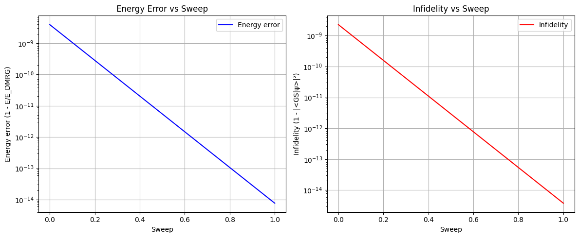
Sweep    Energy         Error       1-Fidelity
------------------------------------------------
    0    -5.08948579    3.956e-09    2.262e-09
    1    -5.08948581    7.661e-15    3.775e-15
11.1.4. 5. Plot Convergence
Plot energy error and infidelity versus sweep number.
fig, (ax1, ax2) = plt.subplots(1, 2, figsize=(12, 5))

ax1.semilogy(sweep_numbers, energy_errors, "b-", label="Energy error")
ax1.set_xlabel("Sweep")
ax1.set_ylabel("Energy error (1 - E/E_DMRG)")
ax1.set_title("Energy Error vs Sweep")
ax1.grid(visible=True)
ax1.legend()

ax2.semilogy(sweep_numbers, infidelities, "r-", label="Infidelity")
ax2.set_xlabel("Sweep")
ax2.set_ylabel("Infidelity (1 - |<GS|ψ>|²)")
ax2.set_title("Infidelity vs Sweep")
ax2.grid(visible=True)
ax2.legend()

plt.tight_layout()
plt.show()