2. Generation of time traces and notion of quasi-static time

In our model, a qubit evolves via a discretized time-dependent Hamiltonian \(h(t) = \epsilon(t) Z\), with \(t=t_s,\dots,N t_s\), where \(t_s\) is the sampling time and acts as our unit of time in our code suite (i.e., \(t_s=1\) in what follows.), and \(N\) is the length of the time trace.

We have three types of noise: quasi-static, white, and pink noise implemented that are defined in spin_pulse.environment.noise.

For a qubit initialized in \(H\ket{0}\), the observable \(X\) will decay in time due to the noise Hamiltonian \(h(t)\).

Repeating this experiment multiple times, we will obtain a Ramsey signal

\[\braket{X(t)}=\frac{1}{2}(1+C)\]

with the Ramsey contrast \(C=\mathbb{E}[e^{-i\sum_{t'\le t}\epsilon(t')}]\), and \(\mathbb{E}\) denotes an ensemble average over multiple random realizations of the time trace.

2.1. Quasi-static noise

In the case of quasi-static noise, we have a time-independent signal \(\epsilon(t)=\epsilon\) where \(\epsilon\) is chosen from a random normal distribution of standard deviation \(\sigma\).

This leads to

\[ C=\mathbb{E}[\exp(-it \epsilon)]=\exp(-t^2\sigma^2/2)=\exp(-t^2/T_2^2) \]

with \(T_2=\sqrt{2}/\sigma\).

Note: the first equality corresponds to the expression of the characteristic function of the normal distribution.

%load_ext autoreload
%autoreload 2
import matplotlib as mpl
import matplotlib.pyplot as plt

from spin_pulse.environment.noise import (
    PinkNoiseTimeTrace,
    QuasistaticNoiseTimeTrace,
    WhiteNoiseTimeTrace,
)

mpl.rcParams["font.size"] = 20

duration = 2**18
segment_duration = 2**8
T2S = 100
time_trace = QuasistaticNoiseTimeTrace(T2S, duration, segment_duration)
time_trace.plot(n_max=2000)
# plt.savefig('../paper/fig3a.pdf',bbox_inches="tight")

ramsey_duration = segment_duration
time_trace.plot_ramsey_contrast(ramsey_duration)
# plt.savefig("fig3d.pdf", bbox_inches="tight")

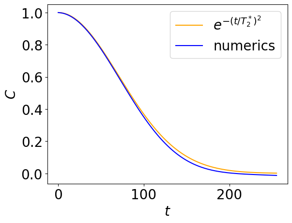
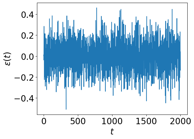
2.2. White noise

In the case of white noise, we have a time-dependent signal where \(\epsilon(t)\) where \(\epsilon(t)\) is chosen from a random normal distribution of standard deviation \(\sigma\).

\[C=\mathbb{E}[\exp(-i\epsilon(1))]^t=\exp(-t\sigma^2/2)=\exp(-t/T_2)\]

with \(T_2=2/\sigma^2\). Remember that the code is expressed in the unit of discretization time \(t_s\), so we have \(T_2=2t_s/\sigma^2\) in SI units.

time_trace = WhiteNoiseTimeTrace(T2S, duration, 1)
time_trace.plot(n_max=2000)
# plt.savefig("../paper/fig3b.pdf", bbox_inches="tight")

time_trace.plot_ramsey_contrast(ramsey_duration)
# plt.savefig("fig3e.pdf", bbox_inches="tight")

2.3. Pink noise

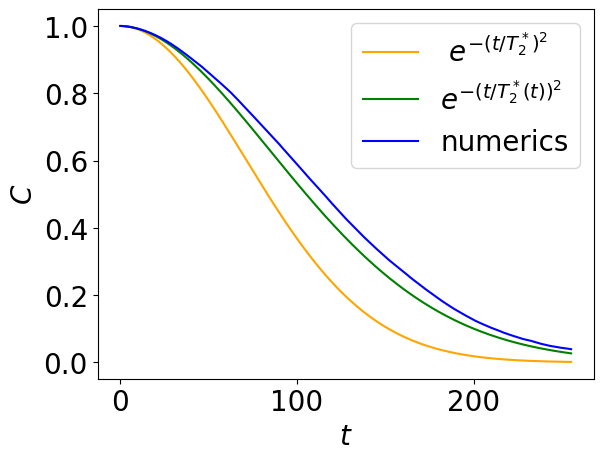
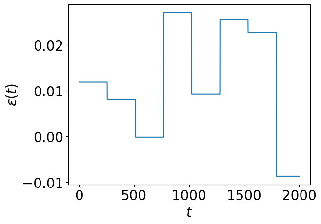
With pink noise, we consider time traces of the form \(\omega(t)=2\pi \sqrt{S_0} g(t)\), where \(g(t)\) is a normalized time trace associated with a Power-Spectral Density \(S_g(f)=1/f\), where \(f\) is the discretized frequency associated with the time vector \(t\) introduced above, and \(S_0\) is the spectral intensity (which has dimension of the square frequency, and is thus written in our code in units of \(t_s^{-2}\))

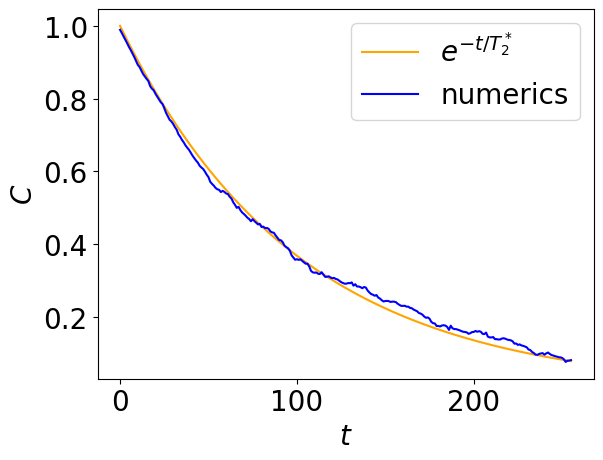
Following Yoneda, et al, 2018, and references therein, the Ramsey contrast can be approximated as follows

\[ C\approx \exp(-t^2/(T_2^\star)^2) \]

with a time-dependent value of the coherence time

\[T_2^\star(t) = \frac{1}{2\pi\sqrt{S_0\log(\frac{1}{f_{\min}t})}}.\]

In the short-time limit, we can assume \(T_2^\star(t)=T_2^\star(1)=T_2^\star\). This gives us a possibility to choose the value of

\[S_0=1/(4\pi^2\log(1/f_{\min})[T_2^\star]^2),\]

for a certain time trace duration \(N\) to achieve a certain value of \(T_2^\star\)

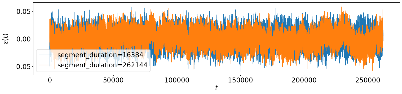
In SpinPulse, the value of \(f_{\min}\) is set as the inverse of the argument segment_duration. Increasing segment_durations incorporates more low-frequency components in the signal.

segment_duration_1 = 2**14
segment_duration_2 = duration
time_trace_1 = PinkNoiseTimeTrace(T2S, duration, segment_duration_1)
time_trace_2 = PinkNoiseTimeTrace(T2S, duration, segment_duration_2)

plt.figure(figsize=(20, 4))
plt.plot(time_trace_1.values)
plt.plot(time_trace_2.values)
plt.xlabel("$t$")
plt.ylabel(r"$\epsilon(t)$")
plt.legend(
    [f"segment_duration={s}" for s in [segment_duration_1, segment_duration_2]], loc=0
)

<matplotlib.legend.Legend at 0x7b1a60a13aa0>

time_trace_2.plot_ramsey_contrast(ramsey_duration)
# plt.savefig("fig3f.pdf", bbox_inches="tight")