5. Average superoperators for noisy gates

In SpinPulse, we can calculate the channel superoperator \(\mathcal{S}=\mathbb{E}[u^*\otimes u]\) representing the average quantum process associated with a quantum circuit.

This can be used to understand the effect of noise on the generation of quantum gates.

The purpose of the present notebook is to calculate \(\mathcal{S}\) via the function mean_channel and represent the corresponding \(\chi\) matrix graphically, for various types of gates and noise. This allows us in particular to benchmark SpinPulse with respect to analytical calculations.

5.1. Idle qubits

We begin by considering single qubit in idle mode, i.e., only subject to Larmor frequency (qubit’s frequency) noise, and consider the following parameters.

n_qb = 1
B0, delta, J_coupling = 0.1, 0.1, 0.005
ramp_dur = 0
T2S = 50
idle_duration = 25

We initialize a qiskit circuit with a single qubit forced to be idle during idle_duration.

%load_ext autoreload
%autoreload 2
import numpy as np
from qiskit import QuantumCircuit, QuantumRegister

delay_circ = QuantumCircuit(QuantumRegister(1))
delay_circ.delay(idle_duration)
delay_circ.draw("mpl")

We load an HardwareSpecs instance, using the hardware parameters defined above, that we will use throughout this example.

from spin_pulse import HardwareSpecs, Shape

hardware_specs = HardwareSpecs(
    num_qubits=n_qb,
    B_field=B0,
    delta=delta,
    J_coupling=J_coupling,
    rotation_shape=Shape.SQUARE,
    ramp_duration=ramp_dur,
)

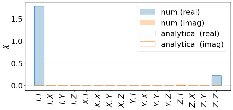
5.1.1. Quasi-static noise

We begin with quasi-static noise and load the corresponding experimental environment. The segment_duration is used to keep the noise constant over the idle duration.

from spin_pulse import ExperimentalEnvironment
from spin_pulse.environment.noise import NoiseType

exp_env_quasistatic = ExperimentalEnvironment(
    hardware_specs=hardware_specs,
    noise_type=NoiseType.QUASISTATIC,
    T2S=T2S,
    duration=1000 * idle_duration,
    segment_duration=idle_duration,
)

The channel superoperator \(\mathcal{S}\) is evaluated by averaging the matrix \(u^*\otimes u\), over each circuit realization \(u\), and for the duration of the experimental environment.

from spin_pulse import PulseCircuit

pulse_circ_quasistatic = PulseCircuit.from_circuit(delay_circ, hardware_specs)
channel_quasistatic = pulse_circ_quasistatic.mean_channel(exp_env_quasistatic)

As described in our publication, the superoperator can be calculated analytically

\[ \mathcal{S}=\frac{1+C}{2}(\mathbf{1}\otimes \mathbf{1}) +\frac{1-C}{2}(Z\otimes Z) \]

with Ramsey contrast \(C=\exp\left(-t^2/(T_2^*)^2\right)\).

The function plot_chi_matrix represents the corresponding \(\chi\) matrices, numerically and analytically calculated. The numerical results closely match the analytical predictions.

from spin_pulse.characterization.average_superop import (
    get_superop_from_paulidict,
    plot_chi_matrix,
)


def contrast_channel(C):
    return get_superop_from_paulidict({"II": (1 + C) / 2, "ZZ": (1 - C) / 2})


C_quasistatic = np.exp(-(idle_duration**2 / T2S**2))

fig = plot_chi_matrix(
    {"num": channel_quasistatic, "analytical": contrast_channel(C_quasistatic)}
)
# fig.savefig('../paper/fig4a.pdf',bbox_inches='tight')

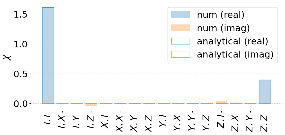
5.1.2. White noise

We proceed similarly with white noise, where analytical calculations predict a Ramsey contrast of the form \(C(t)=\exp\left(-t/T_2^*\right)\). Again, the numerical results closely match the analytical predictions.

exp_env_white = ExperimentalEnvironment(
    hardware_specs=hardware_specs,
    noise_type=NoiseType.WHITE,
    T2S=T2S,
    duration=1000 * idle_duration,
    segment_duration=1,
)

pulse_circ_white = PulseCircuit.from_circuit(delay_circ, hardware_specs)
channel_white = pulse_circ_white.mean_channel(exp_env_white)

C_white = np.exp(-idle_duration / T2S)
fig = plot_chi_matrix({"num": channel_white, "analytical": contrast_channel(C_white)})
# fig.savefig('../paper/fig4b.pdf',bbox_inches='tight')

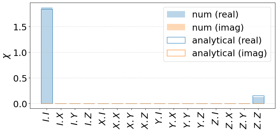
5.1.3. Pink noise

Finally with pink noise, we obtain the superoperator.

exp_env_pink = ExperimentalEnvironment(
    hardware_specs=hardware_specs,
    noise_type=NoiseType.PINK,
    T2S=T2S,
    duration=1000 * idle_duration,
    segment_duration=1000 * idle_duration,
)
pulse_circ_pink = PulseCircuit.from_circuit(delay_circ, hardware_specs)
channel_pink = pulse_circ_pink.mean_channel(exp_env_pink)

In this case, we have a Ramsey contrast \(C(t)\approx \exp\left(-t^2/{T_2^*(t)}^2\right)\) with

\[ T_2^*(t) = T_2^*\sqrt{\frac{\log(1/(f_{\min}t))}{\log(1/f_{\min})}} \]

where \(T_2^*\) is set by the parameter T2S, and \(f_{\min} = (\text{segment\_duration})^{-1}\).

T2_t = T2S / np.sqrt(
    np.log(exp_env_pink.segment_duration / idle_duration)
    / np.log(exp_env_pink.segment_duration)
)

C_pink = np.exp(-(idle_duration**2) / (T2_t**2))
fig = plot_chi_matrix({"num": channel_pink, "analytical": contrast_channel(C_pink)})
# fig.savefig('../paper/fig4c.pdf',bbox_inches='tight')

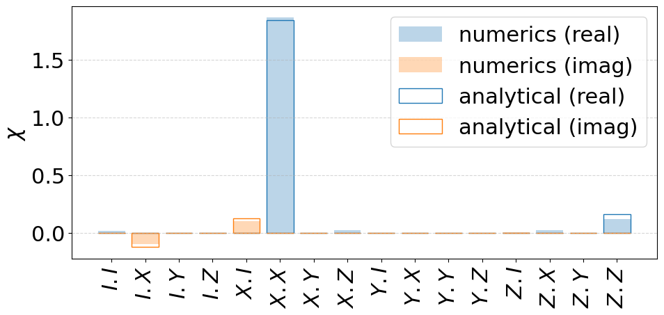
5.2. Single-qubit \(X\) Gate

Let us consider the effect of noise during application of a quantum gate, here \(X=R_X(\pi)\) gate.

x_circ = QuantumCircuit(QuantumRegister(1))
x_circ.rx(np.pi, 0)

pulse_circ_x = PulseCircuit.from_circuit(x_circ, hardware_specs)

5.2.1. Quasi-static noise

We first calculate numerically the superoperator describing the quantum process in presence of quasi-static noise.

exp_env = ExperimentalEnvironment(
    hardware_specs=hardware_specs,
    noise_type=NoiseType.QUASISTATIC,
    T2S=T2S,
    duration=1000
    * pulse_circ_x.duration,  # we take the quasi-static duration to be exactly the circuit duration
    segment_duration=pulse_circ_x.duration,
)


channel_x_quasistatic = pulse_circ_x.mean_channel(exp_env)

Analytically, we can calculate the superoperator, in leading order in \(\sigma=\sqrt{2}/T_2^*\), c.f., our publication.

sigma = exp_env.time_traces[0].sigma
x_chan_pauli = {
    "XX": 1 - sigma**2 / B0**2,
    "IX": 1j * np.pi * sigma**2 / (4 * B0**2),
    "XI": -1j * np.pi * sigma**2 / (4 * B0**2),
    "ZZ": sigma**2 / B0**2,
}
channel_x_quasistatic_analytics = get_superop_from_paulidict(x_chan_pauli)
fig = plot_chi_matrix(
    {"numerics": channel_x_quasistatic, "analytical": channel_x_quasistatic_analytics}
)
# fig.savefig('../paper/fig4d.pdf',bbox_inches='tight')

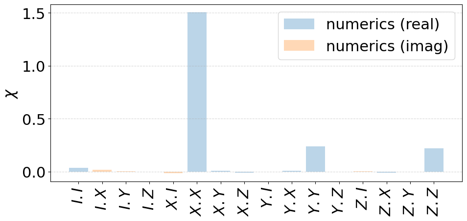
5.2.2. White noise

With white noise, we do not have an analytical expression for the superoperator.

exp_env = ExperimentalEnvironment(
    hardware_specs=hardware_specs,
    noise_type=NoiseType.WHITE,
    T2S=T2S,
    duration=2**14,
    segment_duration=1,
)

pulse_circ_x = PulseCircuit.from_circuit(x_circ, hardware_specs)
channel_x_white = pulse_circ_x.mean_channel(exp_env)

fig = plot_chi_matrix({"numerics": channel_x_white})
# fig.savefig('../paper/fig4e.pdf',bbox_inches='tight')

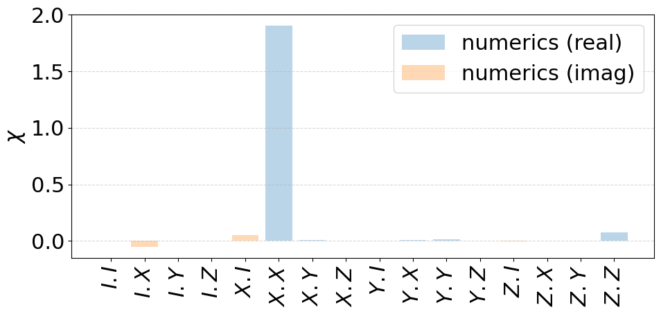
5.2.3. Pink Noise

Finally, with pink noise, we realize that the superoperator has support on similar operators as for quasi-static noise.

exp_env = ExperimentalEnvironment(
    hardware_specs=hardware_specs,
    noise_type=NoiseType.PINK,
    T2S=T2S,
    duration=2**14,
    segment_duration=2**14,
)

pulse_circ_x = PulseCircuit.from_circuit(x_circ, hardware_specs)
channel_x_pink = pulse_circ_x.mean_channel(exp_env)

fig = plot_chi_matrix({"numerics": channel_x_pink})
# fig.savefig('../paper/fig4f.pdf',bbox_inches='tight')

5.3. The two-qubit \(R_{ZZ}\) gate under Larmor frequency (qubit’s frequency) noise.

Our analysis of the two qubit gate begins by redefining the parameters of the hardware, and the pulse circuit associated with an \(R_{ZZ}(\pi/2)\) gate.

hardware_specs = HardwareSpecs(
    num_qubits=2,
    B_field=B0,
    delta=delta,
    J_coupling=J_coupling,
    rotation_shape=Shape.SQUARE,
    ramp_duration=ramp_dur,
)

circ_2q = QuantumCircuit(QuantumRegister(2))
circ_2q.rzz(np.pi / 2, 0, 1)
isa_circ_2q = hardware_specs.gate_transpile(circ_2q)

pulse_circ_2q = PulseCircuit.from_circuit(isa_circ_2q, hardware_specs)

We also define three experimental environments corresponding to quasi-static, white and pink noise. Compared to the single qubit case presented above, we increase the value of \(T_2^*\), to obtain reasonable gate fidelities for the two qubit gate (which is here 10 times slower than the one qubit gate).

T2S = 1000

exp_env_coh = ExperimentalEnvironment(
    hardware_specs=hardware_specs,
    noise_type=NoiseType.QUASISTATIC,
    T2S=T2S,
    duration=1000 * pulse_circ_2q.duration,
    segment_duration=pulse_circ_2q.duration,
)

exp_env_white = ExperimentalEnvironment(
    hardware_specs=hardware_specs,
    noise_type=NoiseType.WHITE,
    T2S=T2S,
    duration=1000 * pulse_circ_2q.duration,
    segment_duration=1,
)

exp_env_pink = ExperimentalEnvironment(
    hardware_specs=hardware_specs,
    noise_type=NoiseType.PINK,
    T2S=T2S,
    duration=1000 * pulse_circ_2q.duration,
    segment_duration=1000 * pulse_circ_2q.duration,
)

We now define a function that calculates the relative superoperator \(\mathcal{S}\mathcal{S_0}^\dagger\) to the ideal channel \(S_0\) (corresponding to an ideal \(R_{ZZ}\) gate). The graphical representation of \(\chi\) matrix of the relative superoperator will be easier to understand. We also extract the fidelity directly from the superoperator.

from qiskit.quantum_info import Operator, SuperOp, average_gate_fidelity


def get_relative_channel(pulse_circ, exp_env):
    channel = pulse_circ.mean_channel(exp_env)
    relative_channel = channel.compose(SuperOp(pulse_circ.original_circ).adjoint())
    fidelity = average_gate_fidelity(channel, Operator(pulse_circ.original_circ))

    return relative_channel, fidelity

channels = []
fidelities = []
for exp_env in [exp_env_coh, exp_env_white, exp_env_pink]:
    results = get_relative_channel(pulse_circ_2q, exp_env)
    channels.append(results[0])
    fidelities.append(results[1])
print("Fidelities ", fidelities)

Fidelities  [0.9988147742473437, 0.7640197813090123, 0.9946581098869455]

As discussed in our publication, we can understand analytically the fact that the gate is much more robust against quasi-static, and pink noise, compared to white noise. The relative superoperator can be expressed as

\[ \mathcal{S}S_0^\dagger = \mathcal{S}_e\otimes \mathcal{S}_e \]

with

\[ \mathcal{S}_e=\frac{1+C_e}{2}(\mathbf{1}\otimes \mathbf{1}) +\frac{1-C_e}{2}(Z\otimes Z) \]

and \(C_e\) is the Ramsey contrast associated with spin-echo (see publication). We have \(C_e(t)=1\) for quasi-static noise,

\[C_e(t)=\exp(-t/T_2^*)\]

for white noise.

For pink noise, we do not have a analytical expression, but expect

\[C_e(t)\gg \exp(-t^2/(T_2^*)^2)\]

because our gates involve a spin echo sequence.

# White noise
# fig = plot_chi_matrix({"num": channels[0]}, threshold=1e-2)
# fig.savefig('../paper/fig4g.pdf',bbox_inches='tight')

Let us check this expression for white noise, defining the spin-echo Ramsey contrast and the corresponding relative channel

C_se = np.exp(-pulse_circ_2q.duration / T2S)
channel_white = contrast_channel(C_se).tensor(contrast_channel(C_se))

fig = plot_chi_matrix(
    {"num": channels[1], "analytical": channel_white},
    threshold=1e-2,
)
# fig.savefig('../paper/fig4h.pdf',bbox_inches='tight')

print("Numerical fidelity ", fidelities[1])
print("Analytical fidelity ", (1 + 4 * C_se) / 5)

Numerical fidelity  0.7640197813090123
Analytical fidelity  0.7492818664338408

Thus, in the case of white noise, the numerical results closely match the analytical predictions for both the \(\chi\)-matrix components and the operation fidelity.

# pink noise
# fig = plot_chi_matrix({"num": relative_channel_2q[2]}, threshold=1e-2)
# fig.savefig('../paper/fig4i.pdf',bbox_inches='tight')

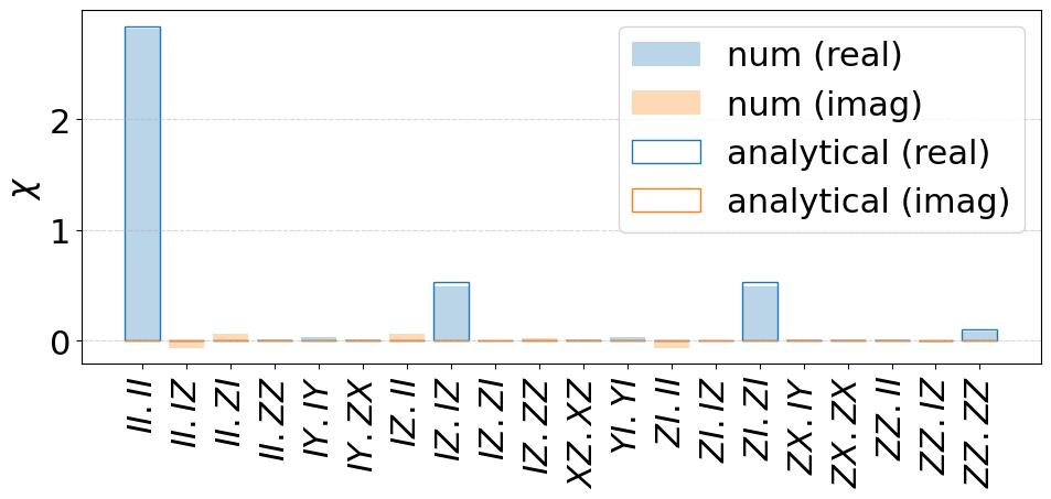
5.4. The two-qubit \(R_{ZZ}\) gate under gate exchange noise

Finally we consider the effect of gate exchange noise, by setting the value of \(T_J^*\ll T_2^*\), and compare the superoperator, with the one obtained analytically.

T2S = 1_000_000
TJS = 500

exp_env = ExperimentalEnvironment(
    hardware_specs=hardware_specs,
    noise_type=NoiseType.QUASISTATIC,
    T2S=T2S,
    duration=1000 * pulse_circ_2q.duration,
    segment_duration=pulse_circ_2q.duration,
    TJS=TJS,
)

channel, fidelity = get_relative_channel(pulse_circ_2q, exp_env)

pulse_circ_2q.plot()

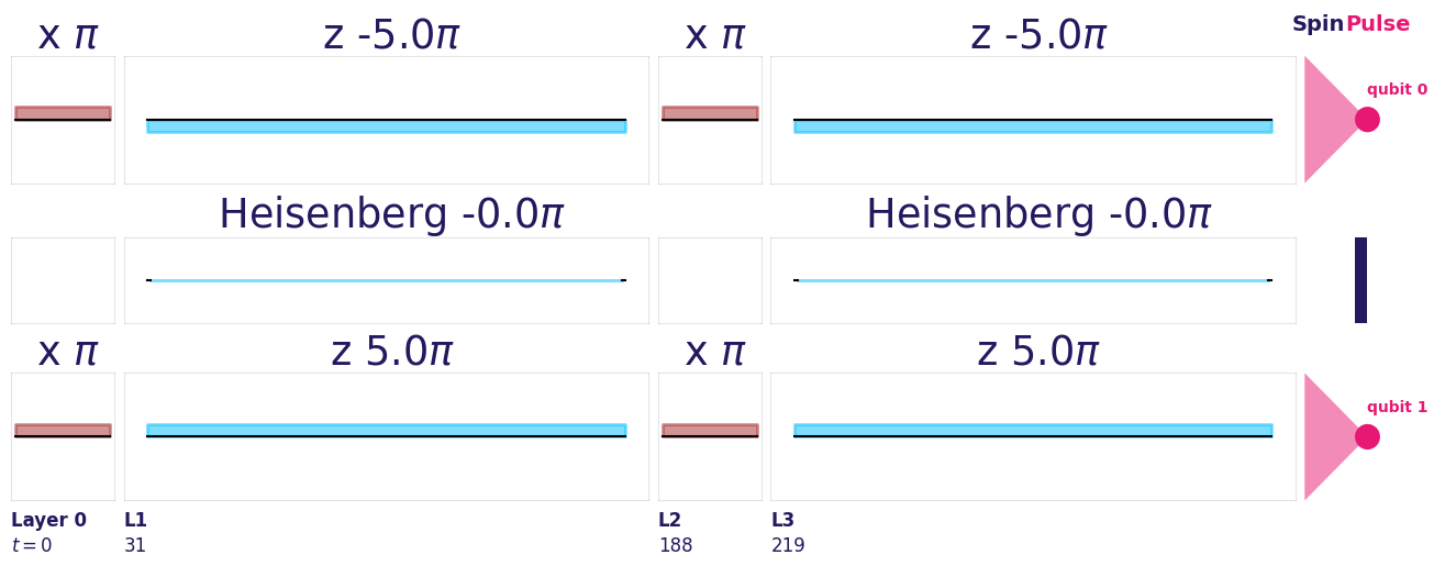
twoq_duration = (
    2
    * pulse_circ_2q.pulse_layers[1]
    .twoq_pulse_sequences[0]
    .pulse_instructions[1]
    .duration
)  # Duration of the two qubit gate

C = np.exp(-(twoq_duration**2) / TJS**2)

twoq_contrast_superop = get_superop_from_paulidict(
    {"IIII": (1 + C) / 2, "ZZZZ": (1 - C) / 2}
)
fig = plot_chi_matrix(
    {"num": channel, "analytical": twoq_contrast_superop}, threshold=1e-2
)

fidelity_analytics = (2 + C) / 3
print("Fidelity ", fidelity)
print("Fidelity (analytics) ", fidelity_analytics)

Fidelity  0.8722776070011851
Fidelity (analytics)  0.8913650513317535

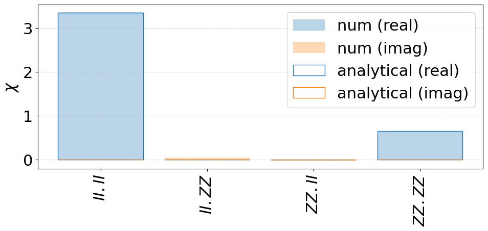
Thus, under quasi-static noise on the \(J\) coupling, the numerical results are in good agreement with the analytical predictions for both the \(\chi\)-matrix components and the operation fidelity, although little deviations from the analytical case are observed.