6. Noise-accurate simulation of the Bernstein–Vazirani algorithm

The Bernstein–Vazirani (BV) algorithm [Bernstein, Vazirani, 1993] finds a secret bitstring \(s\in\{0, 1\}^n\), knowing the function \(f(x)=x\cdot s\), where \(\cdot\) denotes the bit-wise dot-product and \(x\in\{0, 1\}^n\).

Assuming we have a black-box oracle computing \(f\), the algorithm finds \(s\) in one call to the oracle, against \(n\) calls for a classical algorithm.

In the following, we will estimate the success probability of the BV algorithms in the presence of noise.

6.1. Transpilation of the algorithm

We start by generating a qiskit circuit implementing the BV algorithm. We use the hidden string to implement the oracle and neglect the consecutive Hadamard gates (\(H^2=\mathbb{1}\)).

This is clearly a toy example, as we use the hidden string to build the circuit. However, this allows us to measure the impact of noise on the result.

%load_ext autoreload
%autoreload 2
import numpy as np
from qiskit.circuit import QuantumCircuit

from spin_pulse import ExperimentalEnvironment, HardwareSpecs, PulseCircuit, Shape
from spin_pulse.environment.noise import NoiseType


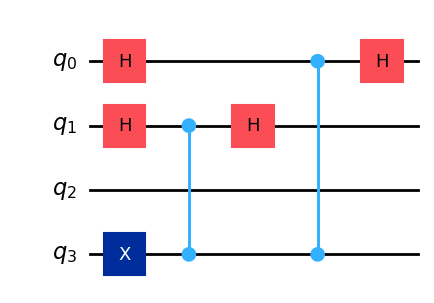
def gen_bv_circ(hidden_string: str | None = None) -> QuantumCircuit:
    """
    Generate the BV circuit using the hidden bitstring to create the oracle.
    We omit the Hadamard gates when there are two consecutive ones on the same qubit.
    """
    num_qubits = len(hidden_string) + 1
    circuit = QuantumCircuit(num_qubits, 0)

    # Initialize the ancilla in |1>
    circuit.x(-1)

    for i in range(num_qubits - 2, -1, -1):
        if hidden_string[num_qubits - 2 - i] == "1":
            circuit.h(i)
            circuit.cz(-1, i)
            circuit.h(i)

    return circuit

# Pick your string
hidden_string = "011"
num_qubits = len(hidden_string) + 1

# Ideal circuit
qc = gen_bv_circ(hidden_string)
qc.draw("mpl")

We first define our hardware specifications and use them to transpile the qiskit circuit according to our needs. We can apply Dynamical Decoupling (DD) on idle qubits during single-qubit unitaries by specifying the DD scheme in HardwareSpecs.

We then define our PulseCircuits to which we attach the transpiled circuit and the hardware specifications. For the noisy case, we also attach an experimental environment that specifies the noise. Note that we deliberately chose a high level of noise to exhibit the effect of DD even on small circuits.

from spin_pulse import DynamicalDecoupling


def get_hdw_specs(DD):
    return HardwareSpecs(
        num_qubits=num_qubits,
        B_field=0.1,
        delta=0.1,
        J_coupling=0.01,
        rotation_shape=Shape.GAUSSIAN,
        ramp_duration=5,
        coeff_duration=5,
        dynamical_decoupling=DD,
        optim=1,
    )


hardware_specs = get_hdw_specs(None)
hardware_specs_DD = get_hdw_specs(DynamicalDecoupling.FULL_DRIVE)

# ISA circuit
isa_qc_bv = hardware_specs.gate_transpile(qc)

# Pulse circuit without noise
pulse_qc_bv_noiseless = PulseCircuit.from_circuit(isa_qc_bv, hardware_specs)

6.2. Noise simulations

Let’s define the duration of our ExperimentalEnvironment such that it is \(n_\text{samples}\) times longer than the circuit duration. This will provide us \(n_\text{samples}\) noisy circuit instances to work with.

n_samples = 500
duration = pulse_qc_bv_noiseless.duration * n_samples

exp_env = ExperimentalEnvironment(
    hardware_specs=hardware_specs,
    noise_type=NoiseType.PINK,
    T2S=500,
    duration=duration,
    segment_duration=duration,
    only_idle=False,
)

# Pulse circuit with noise
pulse_qc_bv_noisy = PulseCircuit.from_circuit(
    isa_qc_bv, hardware_specs, exp_env=exp_env
)

# ISA circuit with DD
isa_qc_bv_DD = hardware_specs_DD.gate_transpile(qc)
# Pulse circuit with noise and DD
pulse_qc_bv_noisy_DD = PulseCircuit.from_circuit(
    isa_qc_bv_DD, hardware_specs_DD, exp_env=exp_env
)

There exist two equivalent solutions (in the limit of an infinite number of samples) to compute our success probability.

We can simulate an experiment that performs a bitstring measurement on each realization of the noisy circuit. Averaging over multiple realizations gives the probability distribution \(P(s)=\bra{s}\rho_f\ket{s}\), where \(\rho_f\) is the density matrix of the system after running the algorithm. In particular, for \(s=s_0\) where \(s_0\) denotes the hidden string, we obtain the success probability of the algorithm.

Alternatively, noting that

\[\rho_f=\mathbb{E}_u\left[u\ket{0^{\otimes N}}\bra{0^{\otimes N}} u^\dagger\right],\]

where \(u\) are the matrices representing the noisy realizations of the quantum circuit, we can recast the success probability as

\[ P(s_0)=\mathbb{E}_u\left[ \left|\bra{s_0}u\ket{0^{\otimes N}}\right|^2\right],\]

and estimate it numerically by calculating the matrices \(u\) explicitely, and averaging the overlap \(\left|\bra{s_0}u\ket{0^{\otimes N}}\right|^2\) over many noisy circuit realizations.

6.2.1. Estimating the success probability by simulating an experiment

The first option is implemented by the method run_experiment of the PulseCircuit class. It executes a single-shot measurement on each noisy instance of the circuit that can be created using the given ExperimentalEnvironment. Simulations are performed using Matrix Product State (MPS) implementation by qiskit_aer.

print("Hidden string ", hidden_string)
print("Expected output in the counts ", "1" + hidden_string)

counts_pulse_qc_bv_noisy = pulse_qc_bv_noisy.run_experiment(exp_env)
print(
    "P_sucess_noise=",
    counts_pulse_qc_bv_noisy["1" + hidden_string]
    / sum(counts_pulse_qc_bv_noisy.values()),
)

counts_pulse_qc_bv_noisy_DD = pulse_qc_bv_noisy_DD.run_experiment(exp_env)
print(
    "P_sucess_noise_DD=",
    counts_pulse_qc_bv_noisy_DD["1" + hidden_string]
    / sum(counts_pulse_qc_bv_noisy_DD.values()),
)

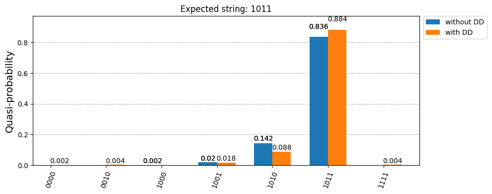
Hidden string  011
Expected output in the counts  1011

P_sucess_noise= 0.836

P_sucess_noise_DD= 0.884

We can visualize the results with plot_histogram provided by qiskit. We observe that DD brings a significant improvement.

from qiskit.visualization import plot_histogram


def normalize_counts(counts):
    tot_sum = sum(counts.values())
    return {k: v / tot_sum for k, v in counts.items()}


normalized_counts_pulse_qc_bv_noisy = normalize_counts(counts_pulse_qc_bv_noisy)
normalized_counts_pulse_qc_bv_noisy_DD = normalize_counts(counts_pulse_qc_bv_noisy_DD)
plot_histogram(
    [normalized_counts_pulse_qc_bv_noisy, normalized_counts_pulse_qc_bv_noisy_DD],
    legend=["without DD", "with DD"],
    title=f"Expected string: 1{hidden_string}",
    figsize=(10, 4),
)

6.2.2. Estimating the success probability by computing the overlap with the hidden bitstring

The second option consists in computing the overlap \(\left|\bra{s_0}u\ket{0^{\otimes N}}\right|^2\) between the hidden bitstring and the state obtained after applying the circuit to \(\ket{0^{\otimes N}}\). To take into account the variability of the noise, we compute this overlap for as many noisy instances of the circuit as ExperimentalEnvironment can create, and we take the average. This is done by calling averaging_over_samples, giving in argument the function my_success_probability_overlap that computes the previously mentioned overlap.

In the present case, the overlap is simply the element in the \(i\)-th row and first column of the unitary operator describing the circuit, with \(i\) the integer representation of “1” followed by the hidden bitstring.

from qiskit.quantum_info import Operator


def my_success_probability_overlap(pulse_qc, hidden_string):
    overlap = np.array(Operator.from_circuit(pulse_qc.to_circuit()))[
        int("1" + hidden_string, 2), 0
    ]
    return np.real(overlap * overlap.conjugate())

We repeat the process several times for different noisy circuit instances to obtain an average. It is done using the averaging_over_samples method of PulseCircuit. We obtain, up to statistical errors, the same values as with the previous method.

print("Hidden string ", hidden_string)
print("Expected output in the counts ", "1" + hidden_string)
print(
    "P_sucess_noiseless=",
    my_success_probability_overlap(pulse_qc_bv_noiseless, hidden_string),
)

print(
    "P_sucess_noise=",
    pulse_qc_bv_noisy.averaging_over_samples(
        my_success_probability_overlap, exp_env, hidden_string
    ),
)

print(
    "P_sucess_noise_DD=",
    pulse_qc_bv_noisy_DD.averaging_over_samples(
        my_success_probability_overlap, exp_env, hidden_string
    ),
)

Hidden string  011
Expected output in the counts  1011
P_sucess_noiseless= 0.9999983912873237

P_sucess_noise= 0.8164334242339304

P_sucess_noise_DD= 0.8957357429179306

Again, we observe that DD brings a significant improvement.