4. Coherence times via Ramsey and Spin Echo experiments

In our model, a qubit evolves via a discretized time-dependent Hamiltonian \(h(t) =\frac{ \omega(t)}{2}Z\), with \(t=t_s,\dots,N t_s\), where \(t_s\) is the sampling time and acts as our unit of time in our code suite (i.e., \(t_s=1\) in what follows), and \(N\) is the length of the time trace.

With pink noise, we consider time traces of the form \(\omega(t)=2\pi \sqrt{S_0} g(t)\), where \(g(t)\) is a normalized time trace associated with a Power-Spectral Density \(S(f)=1/f\), where \(f\) is the discretized frequency associated with the time vector \(t\) introduced above, and \(S_0\) is the spectral intensity (which has dimension of the square frequency, and is thus written in our code in units of \(t_s^{-2}\))

In this notebook, we will study how an individual qubit is affected by such noise, in the context of Ramsey and spin echo experiments.

%load_ext autoreload
%autoreload 2
import numpy as np

from spin_pulse import (
    DynamicalDecoupling,
    ExperimentalEnvironment,
    HardwareSpecs,
    Shape,
)
from spin_pulse.environment.noise import NoiseType

num_qubits = 1
B_field, delta, J_coupling = 0.5, 0.5, 0.05
hardware_specs = HardwareSpecs(num_qubits, B_field, delta, J_coupling, Shape.SQUARE)

exp_env = ExperimentalEnvironment(
    hardware_specs=hardware_specs,
    noise_type=NoiseType.PINK,
    T2S=100,
    duration=2**18,
    segment_duration=2**16,
)

We first initialize a Ramsey circuit, that is made of two Hadamard gates interspersed by an Idle layer of parametrized duration.

from spin_pulse.characterization.ramsey import get_ramsey_circuit

duration = 100
ramsey_circuit = get_ramsey_circuit(duration, hardware_specs)
ramsey_circuit.plot(hardware_specs)

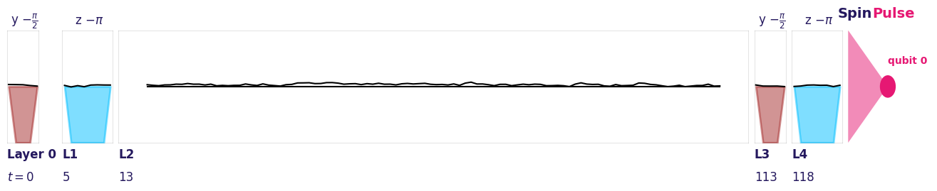
Let us now consider the noisy version of a Ramsey circuit by assigning a noisy time trace of our experimental environment

ramsey_circuit = get_ramsey_circuit(duration, hardware_specs, exp_env=exp_env)
ramsey_circuit.plot(hardware_specs)

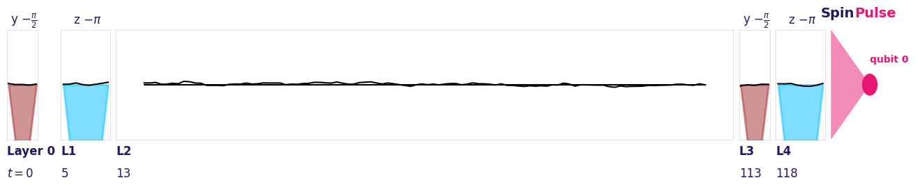
We can produce noisy iterations of the circuit by calling function assign_time_trace repeatedly. Internally, a variable t_lab is used to attach the different time_traces fragments from our experimental environment, and is incremented by the circuit duration. This mimicks an experimental sequence, where a list of circuits is executed sequentially.

print("Lab time after first time_trace assignment", ramsey_circuit.t_lab)
ramsey_circuit.attach_time_traces(exp_env)
print("Lab time after first time_trace assignment", ramsey_circuit.t_lab, "...")
ramsey_circuit.plot()

Lab time after first time_trace assignment 126
Lab time after first time_trace assignment 252 ...

The number of available time trace fragments, which we call samples, is the integer part of the duration of the experimental environment divided by the duration of the circuit.

print(
    "Number of experimentally available samples ",
    ramsey_circuit.circuit_samples(exp_env),
)

Number of experimentally available samples  2080

Using the function get_average_ramsey_contrast, we repeat the circuit over such multiple samples and calculate the average contrast. This uses the function averaging_over_samples that can be used to calculate any averaged quantity of a given function of a pulse_circuit (here the Ramsey contrast).

Here the contrast corresponds to the expectation value of the \(X\) operator after the idle sequence, and can be obtained from computational basis measurements after the second Hamard gate.

from spin_pulse.characterization.ramsey import get_average_ramsey_contrast

durations = np.arange(30, 300, 40, dtype=int)
average_contrast = get_average_ramsey_contrast(hardware_specs, exp_env, durations)

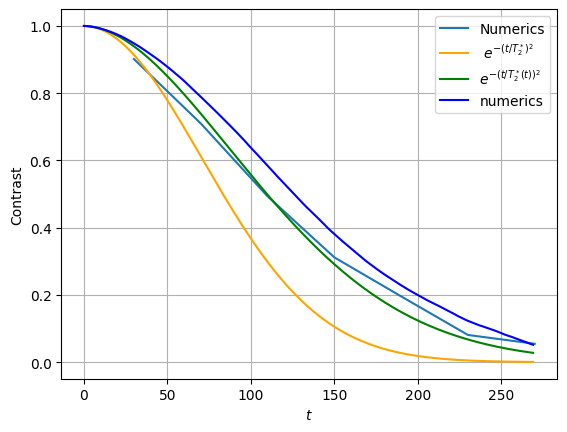
We can compare with the function plot_ramsey_contrast which directly integrates the timetrace values, and also compare with approximate analytical expressions, functions of \(T_2^*\) (that we recall in our publication).

In the plot, the curve entiled “Numerics” correspond to the contrast obtained from get_average_ramsey_contrast, that is calculated from the array durations (see above).

And the curve “numerics” correspond to the contrast obtain from ramsey_contrast in file from src/spin_pulse/environment/noise/noise_time_trace.py.

import matplotlib.pyplot as plt

plt.plot(durations, average_contrast, "-", label="Numerics")
exp_env.time_traces[0].plot_ramsey_contrast(durations[-1])
plt.xlabel("$t$")
plt.ylabel("Contrast")
plt.grid()
plt.legend(loc=0)

<matplotlib.legend.Legend at 0x70c02838a210>

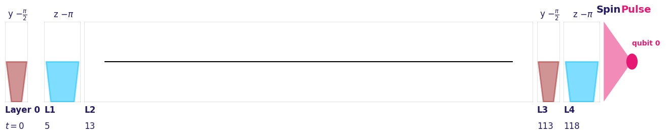
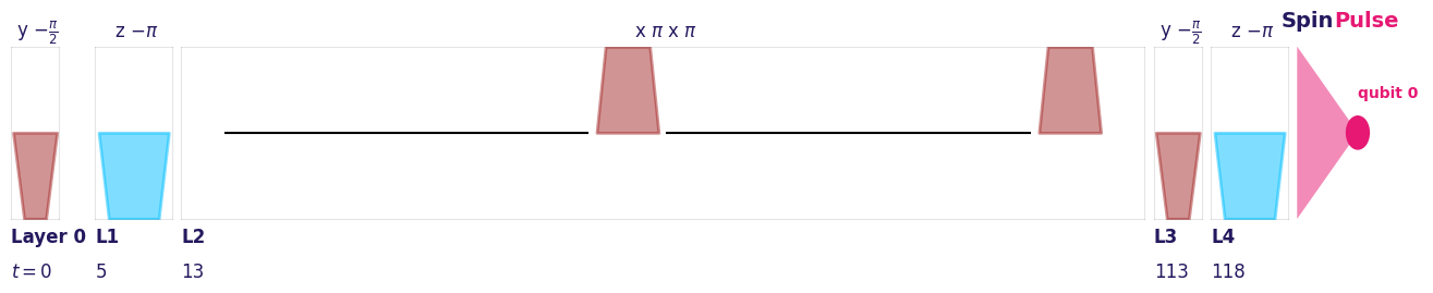
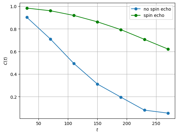
4.1. Spin Echo

Given an Idle time period, we can add two \(X\) pulses to remove low-frequency drifts, and ‘refocus’ our Ramsey signal. The spin-echo sequence can be chosen by redefining our hardware_specs variable.

hardware_specs_se = HardwareSpecs(
    num_qubits,
    B_field,
    delta,
    J_coupling,
    Shape.SQUARE,
    dynamical_decoupling=DynamicalDecoupling.SPIN_ECHO,
)
spinecho_circuit = get_ramsey_circuit(duration, hardware_specs_se)
spinecho_circuit.plot(hardware_specs)

average_spinecho_contrast = get_average_ramsey_contrast(
    hardware_specs_se, exp_env, durations
)

plt.plot(durations, average_contrast, "-o", label="no spin echo")
plt.plot(durations, average_spinecho_contrast, "-o", label="spin echo", color="green")
plt.xlabel("$t$")
plt.ylabel("$C(t)$")
plt.grid()
plt.legend(loc=0)

<matplotlib.legend.Legend at 0x70c028b64620>

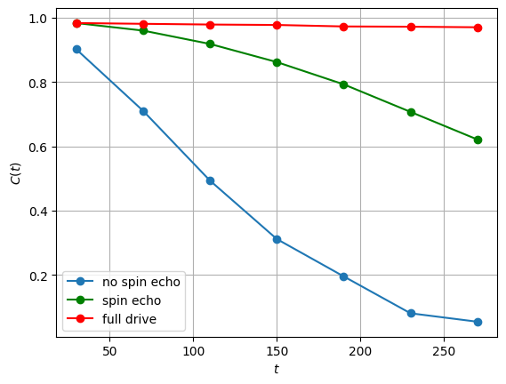
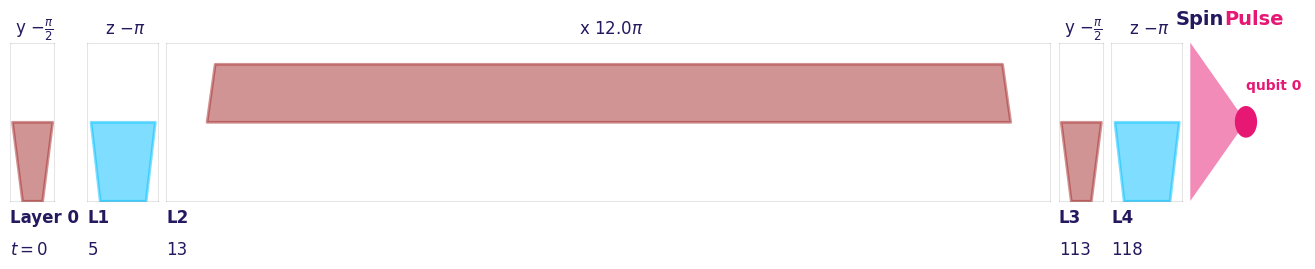
4.2. Full-drive dynamical decoupling

The spin-echo does not remove high-frequency components of the noise signal. To improve on that, we can use a full-drive dynamical decoupling sequence where the qubit is subject to a constant \(X\) field that integrates to a multiple of \(2\pi\).

from spin_pulse import DynamicalDecoupling

hardware_specs_fd = HardwareSpecs(
    1,
    B_field,
    delta,
    J_coupling,
    Shape.SQUARE,
    dynamical_decoupling=DynamicalDecoupling.FULL_DRIVE,
)
fulldrive_circuit = get_ramsey_circuit(duration, hardware_specs_fd)
fulldrive_circuit.plot(hardware_specs)

average_fulldrive_contrast = get_average_ramsey_contrast(
    hardware_specs_fd, exp_env, durations
)

plt.plot(durations, average_contrast, "-o", label="no spin echo")
plt.plot(durations, average_spinecho_contrast, "-o", label="spin echo", color="green")
plt.plot(durations, average_fulldrive_contrast, "-o", label="full drive", color="red")


plt.xlabel("$t$")
plt.ylabel("$C(t)$")
plt.grid()
plt.legend(loc=0)

<matplotlib.legend.Legend at 0x70c0285fa210>